

How to create a pivot table in Excel (step-by-step)
Watch alongside this article
Public YouTube resources matched to this article's topic, functions, and practice goal.


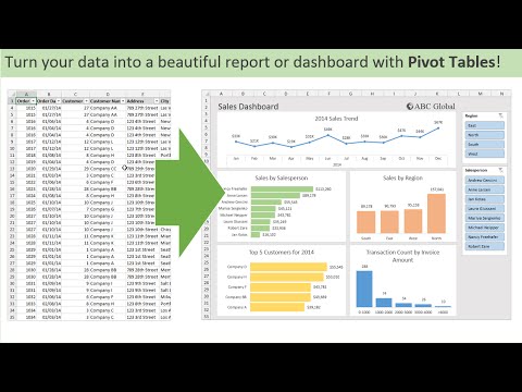
Introduction to Pivot Tables, Charts, and Dashboards in Excel (Part 1)
Excel Campus - Jon
Open on YouTube (opens in a new tab)A pivot table summarizes a big table of raw data — totals, counts, averages — without writing a single formula. You drag fields into place, and it does the math.
Step 1: Prepare your data
Pivot tables need a proper table, not just data that looks organized:
- One row per record, with column headers in the first row
- No blank rows or columns inside the range
- No merged cells
- Each column holds one kind of value (a “Region” column, not a mix of regions and subtotals)
Messy source data is the single biggest cause of pivot table problems — sort this out first and everything downstream gets easier.
Step 2: Insert the pivot table
Click anywhere inside your data, then Insert → PivotTable. Excel guesses the range automatically — confirm it’s correct, choose New Worksheet, and click OK.
Step 3: Build it
A PivotTable Fields pane appears with your column headers listed at the top and four boxes below: Filters, Columns, Rows, and Values.
- Drag a category field (like “Region”) into Rows to group by it
- Drag a number field (like “Revenue”) into Values to total it
- Drag another category (like “Product”) into Columns to break it out side by side
- Drag a field into Filters to add a dropdown that limits the whole table
The pivot table updates instantly as you rearrange fields — this is the part worth just experimenting with.
Step 4: Change how values summarize
By default, numbers get summed and text gets counted. To change that, click the field in the Values box, choose Value Field Settings, and pick Sum, Count, Average, Max, Min, or a few others.
Common mistakes
- “(blank)” showing up as a category — usually means there are empty cells in that column in the source data.
- Forgetting to refresh — a pivot table doesn’t update automatically when the source data changes. Right-click anywhere in it and choose Refresh.
- New rows not appearing after refresh — if you added rows past the original range, refreshing won’t pick them up. Rebuild the source as a proper Excel Table (Insert → Table) first, and the pivot table’s range will expand automatically.
When a formula is enough
For a single number — “total revenue where region is North” — a formula like SUMIFS is often faster than building a whole pivot table. Reach for a pivot table when you need to slice the same data multiple ways, or explore it interactively rather than compute one fixed answer.
Go deeper with this skill
Use PivotTables to explore data quickly while keeping the source table clean and refreshable. For this article, the goal is to practice: A beginner's guide to building your first pivot table: preparing your data, choosing rows and values, and the mistakes that trip up almost everyone.
Practice workbook setup
Prepare a source table with headers, dates, categories, and numeric measures.
Practice workflow
- Convert the source data into an Excel Table before inserting the PivotTable.
- Build one simple summary first, then add filters, slicers, or grouping.
- Change value field settings and number formats so the result matches the question.
- Refresh after changing the source data and confirm new rows appear.
Quality checks
- The source table has no blank header names or merged cells.
- The PivotTable answers a specific question.
- Filters and slicers are visible enough for readers to know what they are seeing.
Common mistakes
- Building pivots from messy ranges instead of clean tables.
- Forgetting to refresh after source changes.
- Counting text fields when a numeric sum was expected.
Next actions
- Add one slicer and one PivotChart to turn the summary into a small report.
- Create a second PivotTable from the same source to answer a different question.
Formula focus: even if this workflow is not formula-heavy, add one check cell that confirms the final output still matches the source data.


