Excel Intermediate Skills

This is the paid upgrade from Excel for Beginners - not a longer version of the same book, but a different kind of book. Instead of resetting the example every chapter, everything here follows one real-feeling small business, Reyes Roastery, through one evolving workbook, from Chapter 1 to the last page. By the end, you will have built - not just read about - a lookup-driven order log, a live dashboard, a Power Query cleanup step, and your first macro, all inside the same file.

Dana Reyes runs Reyes Roastery, a small-batch coffee roaster selling bagged coffee three ways: online, at the Saturday farmers market, and as walk-in pickup from the roastery itself. Dana knows the basics - the free edition’s whole table of contents - but the spreadsheet has started to strain: formulas copied by hand, a growing product list, and a first attempt at “let me just check this in a PivotTable” that didn’t quite work. This book is what Dana does next.

The bonus companion workbook is the same file Dana works in throughout the book - download it now and follow along sheet by sheet as each chapter builds on the last. A one-page completion checklist waits at the very end, worth screenshotting when you get there. (Downloading it needs a free Google sign-in - the book itself you can keep reading right here either way.)

Eleven chapters in four parts, plus a closing bridge chapter. Work through them in order - later chapters lean directly on data and formulas built in earlier ones, the same way real spreadsheets grow.

PART I

A Real Data System

Before Reyes Roastery can analyze anything, its data needs a real structure: named Tables, formulas that look values up instead of retyping them, entry that can't go wrong, and a vocabulary of names instead of bare cell addresses.

1. Meet Reyes Roastery: Setting Up a Multi-Sheet Workbook
2. Smarter Lookups: XLOOKUP, INDEX/MATCH, and Multi-Column Returns
3. Keeping Data Clean at the Source: Data Validation & Drop-Downs
4. Named Ranges and Structured References

1. Meet Reyes Roastery: Setting Up a Multi-Sheet Workbook

After this chapter you’ll be able to: turn a plain list into a real Excel Table, and lay out a workbook across several purpose-built sheets instead of one crowded one.

A spreadsheet that has “grown” instead of been “designed” usually shows it: one giant sheet with product info, orders, and scratch calculations all mixed into whichever columns happened to be free. The fix isn’t complicated - it’s the same idea as a filing cabinet. Give each kind of information its own labeled drawer (sheet), and give the thing everyone else needs to find - the product list - a name, not just a location.

Reyes Roastery’s companion workbook has five sheets: Products (this chapter), Inventory (Chapter 3), Orders (Chapters 2, 4, 5, 6), MonthlyExports (Chapter 9), and Dashboard (Chapters 7-8), plus a NewOrderForm sheet for Chapters 10-11. Every sheet earns its place - none of them is “just in case.”

Start with Products: SKU, Product, Roast, Size, Cost, and Price for the five items Reyes Roastery currently sells. Select the range including headers and press Ctrl+T (or Insert > Table). Give it a real name - the Name Box shows “Table1” by default, so open Table Design (the ribbon tab that appears whenever a cell inside a Table is selected) and rename it to Products in the “Table Name” box on the far left.

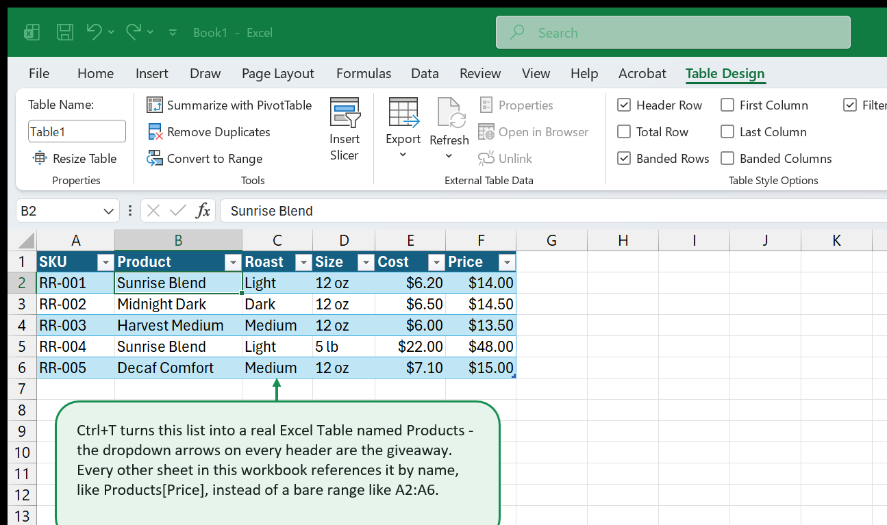
That single rename is what makes every later chapter possible. Once a Table has a name, any formula anywhere in the workbook can reference Products[Price] instead of a bare range like $F$2:$F$6 - and if a new coffee gets added as row 7, every formula referencing Products[Price] already includes it, automatically, with nothing to edit.

2. Smarter Lookups: XLOOKUP, INDEX/MATCH, and Multi-Column Returns

After this chapter you’ll be able to: pull two related values (like a product name and its price) from one lookup formula, and understand the older INDEX/MATCH pattern well enough to read it in an inherited workbook.

The free edition covered VLOOKUP and a single-result XLOOKUP. Here’s the part that usually gets skipped: XLOOKUP’s return_array argument doesn’t have to be one column. Point it at a two-column range, and XLOOKUP returns both values at once, spilling across two cells from a single formula.

Reyes Roastery’s Orders sheet logs every sale by SKU - not by product name or price, since those live in Products and change over time (Dana’s already raised the price on the medium roast twice). Rather than writing one XLOOKUP for Product and a second for Price, one formula does both:

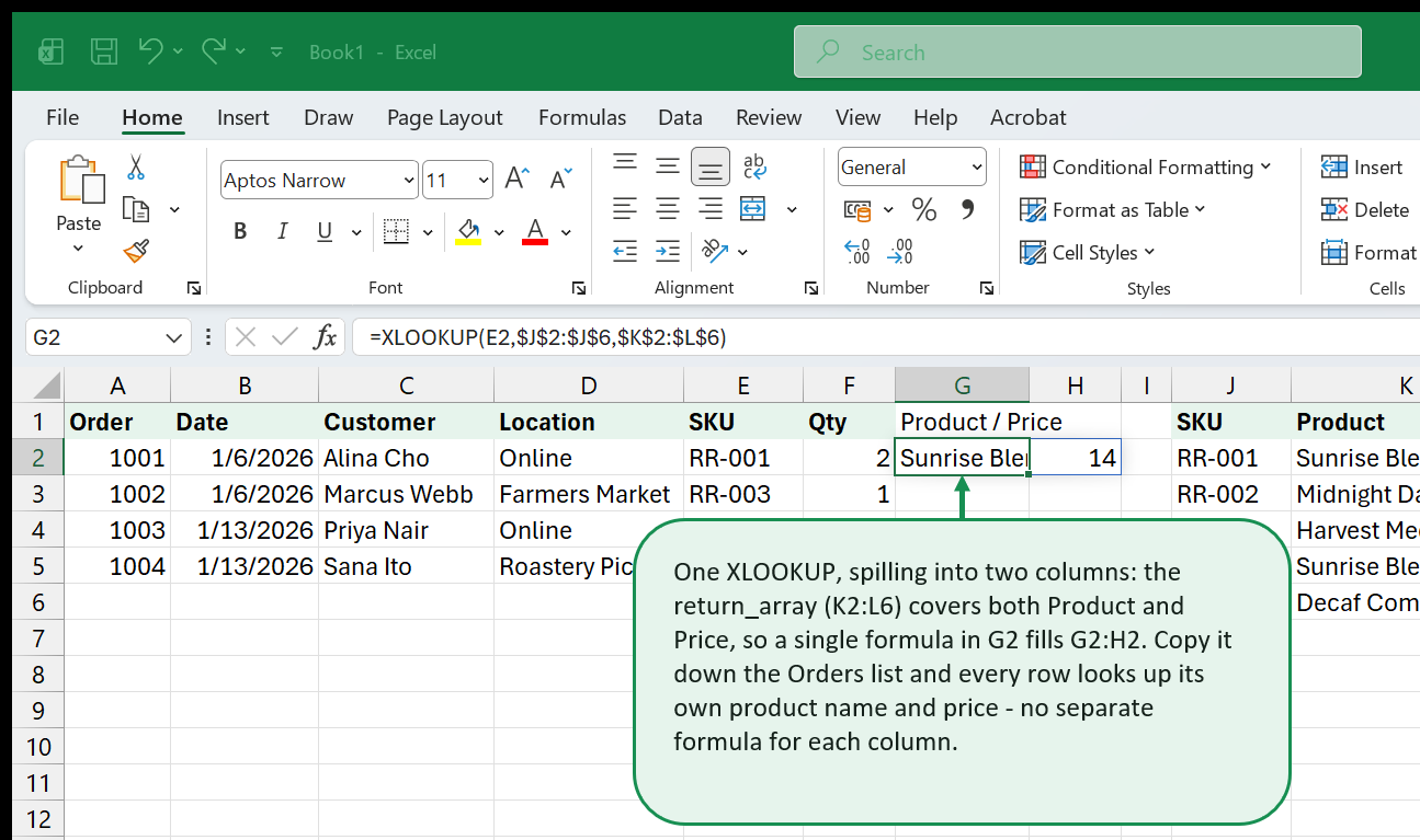
$J$2:$J$6 is the lookup array (SKU) and $K$2:$L$6 is the return array - two full columns, Product and Price. Because the return array is two columns wide, the result is too: one row, two columns, spilling out of G2 into G2:H2. Copy the formula down the Orders list and every row fills in its own product name and price with no separate formula needed for each column.

The older, two-function way to do the same lookup - worth recognizing, since it appears throughout workbooks built before XLOOKUP existed (Excel 2019 and earlier) - combines MATCH (which finds a position) with INDEX (which returns a value at that position):

MATCH(E2,Products[SKU],0) finds where E2’s SKU sits inside the SKU column (the 0 forces an exact match, the INDEX/MATCH equivalent of VLOOKUP’s FALSE); INDEX(Products[Price], ...) then returns the price sitting at that same position. It takes two functions to do what one XLOOKUP does, but it works in every version of Excel, and reads fine once you know the pattern: MATCH finds the row, INDEX fetches the value.

3. Keeping Data Clean at the Source: Data Validation & Drop-Downs

After this chapter you’ll be able to: restrict a cell to a fixed list of valid entries, so bad data never gets typed in the first place.

The free edition’s Chapter 14 covered cleaning up messy data after the fact - TRIM, Remove Duplicates, converting text-that-looks-like-a-number. Data Validation solves a related problem from the other direction: instead of catching mistakes later, it prevents a whole category of them from happening at all.

Reyes Roastery’s Inventory sheet tracks bags on hand per SKU, by location - Roastery, Farmers Market, or Online Warehouse. Typed by hand, “Farmers Market” becomes “farmers market,” “Farmer’s Market,” and “FM” within a week, and every one of those variants breaks a SUMIFS or PivotTable grouping by location later. A dropdown list fixes it at the source: select the Location column, Data tab > Data Validation, Allow: List, and type the three valid values (or point at a range that holds them).

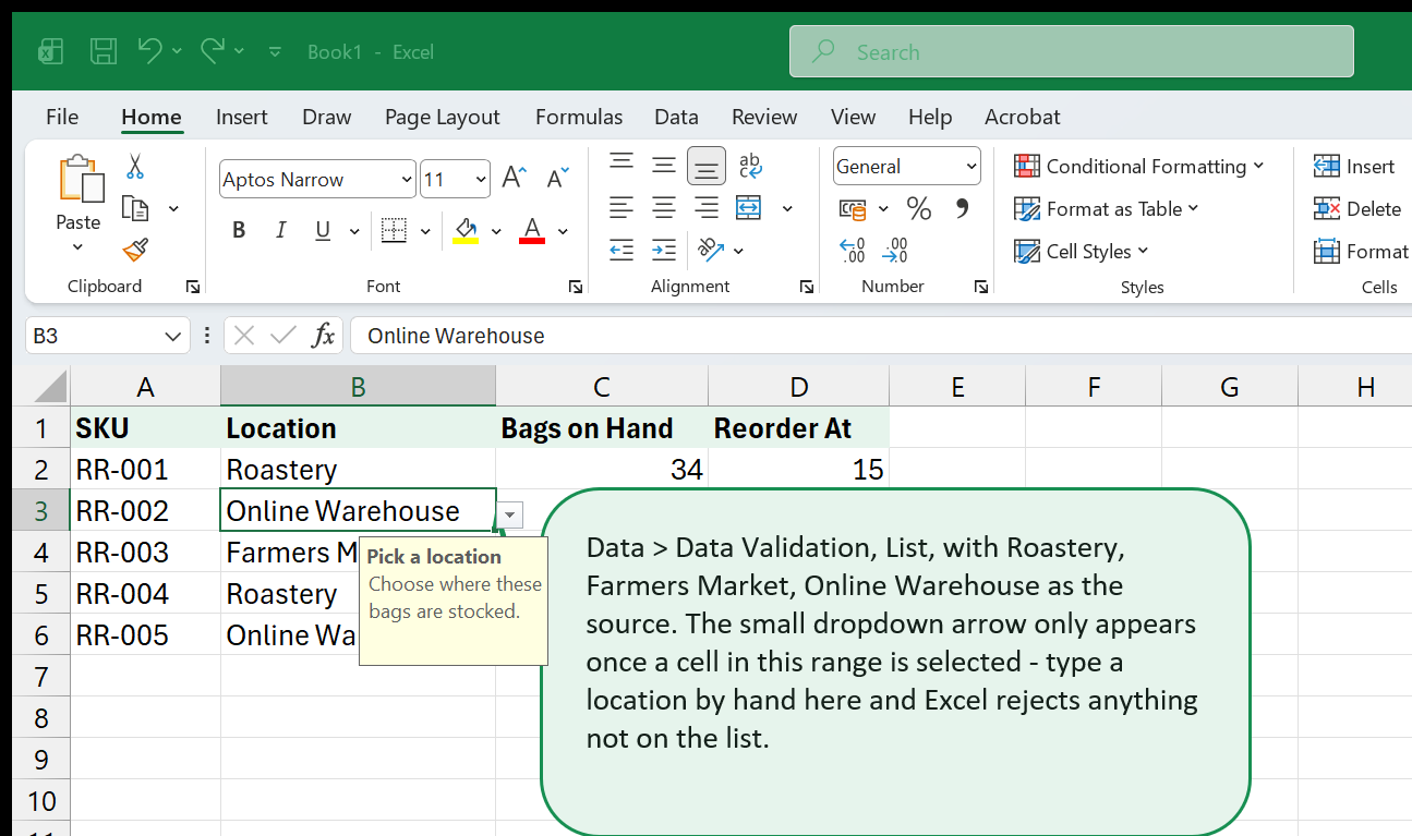
The small dropdown arrow only appears once a cell inside the validated range is selected - it isn’t a permanent visual change to the sheet. Try typing a location by hand that isn’t on the list; Excel’s default “Stop” alert rejects the entry outright rather than letting a near-miss slip through.

4. Named Ranges and Structured References

After this chapter you’ll be able to: give a cell or range a plain-English name and use it inside formulas instead of a bare address.

A Table’s column names (Products[Price]) are one kind of “structured reference.” A named range is the more general version - any cell, range, or even a typed formula, given a name that formulas anywhere in the workbook can use instead of an address like $G$2.

Reyes Roastery offers a small bulk discount: orders of three or more bags get 10% off. That 10% lives in one cell so it can be changed in one place if it ever moves. Select the cell, then Formulas > Define Name (or simpler: click the Name Box directly above the grid, type CaseDiscount, and press Enter) to name it.

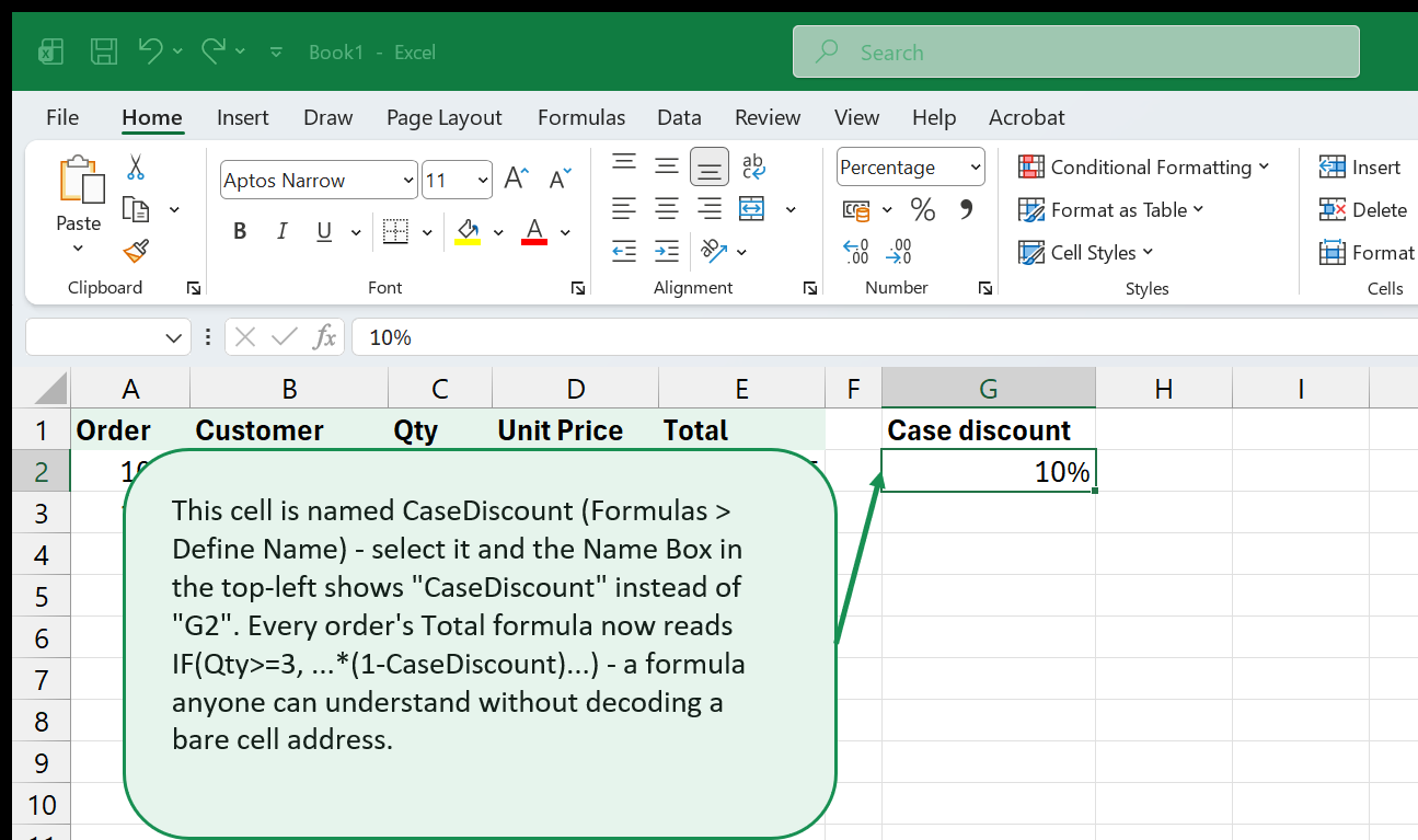
Every order’s Total formula can now read:

instead of the equivalent formula built with $G$2 scattered through it. Both calculate identically - the difference is entirely for a human reading the formula later (including future-you). CaseDiscount says what the number means; $G$2 only says where it lives.

PART II

Analysis at Scale

With clean, named, connected data in place, Reyes Roastery can finally ask real questions of it: which customers, which locations, which totals - without writing a new formula by hand for every answer.

1. Dynamic Arrays: FILTER, SORT, and UNIQUE
2. Multi-Criteria Analysis: SUMIFS, COUNTIFS, and AVERAGEIFS
3. PivotTables, Leveled Up: Grouping, Calculated Fields, and Slicers
4. Building Your First Dashboard

5. Dynamic Arrays: FILTER, SORT, and UNIQUE

After this chapter you’ll be able to: write one formula that spills a whole list of results into neighboring cells automatically, instead of copying a formula down by hand.

Every formula so far has produced one answer per cell. Excel 365’s dynamic array functions break that rule on purpose: a single formula can return many results at once, and Excel “spills” them into the cells below and beside it automatically - visible as a faint blue outline around the whole result while any cell inside it is selected.

UNIQUE(range) returns every distinct value in a range, in the order it first appears. Wrap it in SORT(...) to alphabetize (or numerically sort) the result:

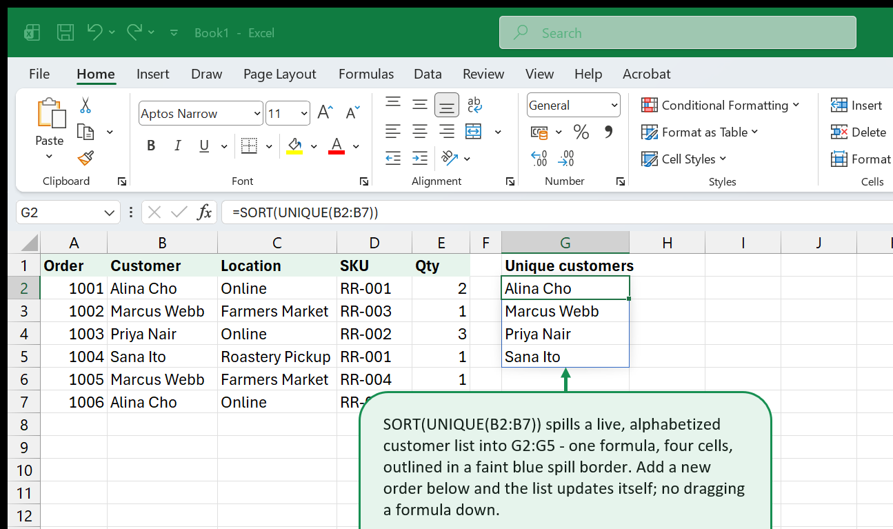
FILTER(range, condition) is the third function in this family - it returns only the rows matching a condition, spilling as many rows as match:

All three - UNIQUE, SORT, FILTER - update automatically the moment the source data changes, exactly like every other formula in this book. Reference the whole spilled result from elsewhere with the spill range operator, a # right after the anchor cell: =COUNTA(K3#) counts every name in the spilled list without you ever hardcoding how many rows that turns out to be.

6. Multi-Criteria Analysis: SUMIFS, COUNTIFS, and AVERAGEIFS

After this chapter you’ll be able to: total or count rows that match more than one condition at once, without a helper column.

SUMIF and COUNTIF (from the free edition) each handle exactly one condition. The moment Reyes Roastery needs “total bags sold at the farmers market” rather than just “total bags sold,” a second condition is required - and that’s what the -IFS family (SUMIFS, COUNTIFS, AVERAGEIFS) is for.

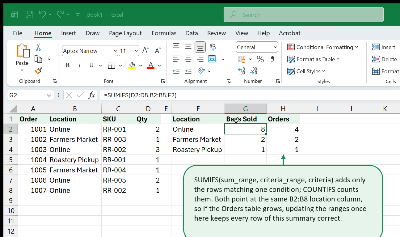
SUMIFS(sum_range, criteria_range1, criteria1, [criteria_range2, criteria2, ...]) - notice the sum range comes first in SUMIFS, the opposite order from SUMIF, which is the single most common typo when upgrading a formula from one condition to several. COUNTIFS follows the same criteria-pair pattern with no sum range at all, since it’s only counting matching rows: =COUNTIFS(B2:B8,F2).

Add a second condition the same way - a third pair of arguments: =SUMIFS(D2:D8,B2:B8,F2,C2:C8,"RR-001") totals bags sold Online and specifically SKU RR-001. AVERAGEIFS follows the identical shape, sum range first, for an average instead of a total.

7. PivotTables, Leveled Up: Grouping, Calculated Fields, and Slicers

After this chapter you’ll be able to: nest two fields inside a PivotTable’s Rows area, and add a slicer for one-click filtering.

The free edition’s Chapter 16 built a single-level PivotTable - one field in Rows, one in Values. The real jump in usefulness comes from nesting a second field, and from replacing a plain filter dropdown with a slicer.

Build a PivotTable from Reyes Roastery’s order data (Insert > PivotTable, source = the Orders table). Drag Location into Rows first, then drag Product into Rows underneath it - Excel nests Product inside each Location group automatically, no extra setup required.

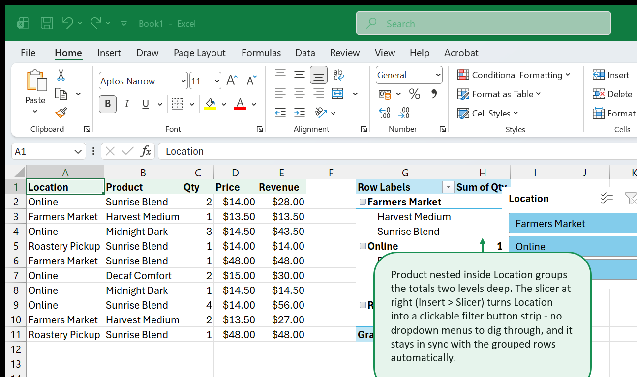
Insert > Slicer, then check Location, turns that field into a strip of clickable buttons - click “Farmers Market” and the whole PivotTable (and any chart built from it) filters instantly, with the currently-selected button visually highlighted. It’s the same filtering a dropdown arrow on the Location field already gave you, just visible at a glance instead of hidden behind a click.

A PivotTable is a snapshot, not a live formula - it does not notice new source rows on its own. Right-click anywhere inside it and choose Refresh (or Data > Refresh All) any time the underlying Orders table grows, or the totals will quietly go stale.

8. Building Your First Dashboard

After this chapter you’ll be able to: combine KPI cards, a chart, and conditional formatting on one sheet, all pulling live from the same source data.

A dashboard isn’t a special Excel feature - it’s a plain worksheet, deliberately laid out so the most important numbers are readable at a glance, fed entirely by formulas so nothing on it ever needs to be updated by hand.

Reyes Roastery’s Dashboard sheet has three KPI cards - merged, bordered cells with a large bold number - each driven by one formula against the Orders table:

Total Revenue, Total Orders, and Average Order Value, in that order - the third KPI is just the first divided by the second, referencing the other two cards’ own cells rather than recalculating from scratch.

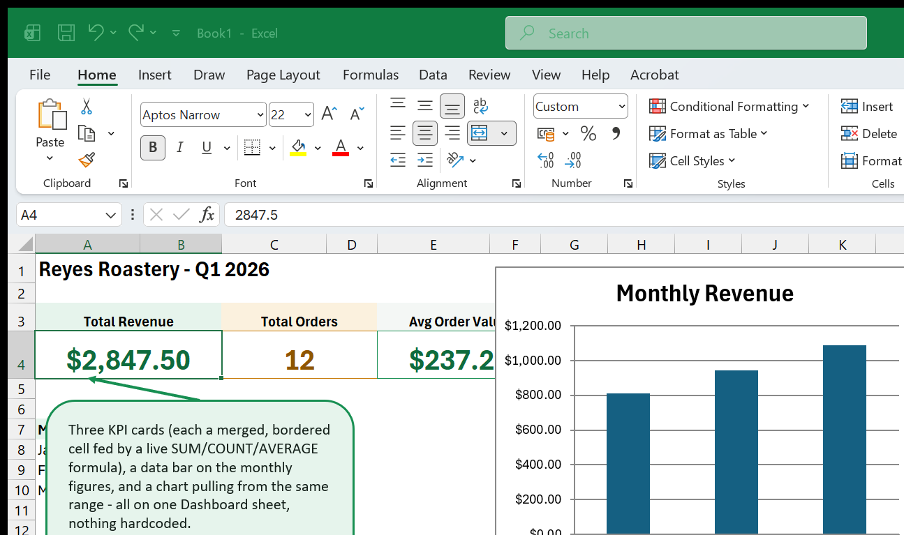
Beside the KPI cards, a small Month/Revenue table (Jan, Feb, Mar) uses SUMPRODUCT to total each month’s orders directly from the Orders table’s Date and Total columns, then feeds a column chart - Insert > Chart, same as the free edition’s Chapter 15, just pointed at a formula-built range instead of typed-in numbers. A data bar (Home > Conditional Formatting > Data Bars) on that same table turns the numbers into an instant mini bar chart with no separate chart object.

PART III

Automating the Busywork

The last three chapters cover the natural next step past formulas: importing and cleaning data without retyping it, recording a first macro, and wiring a small entry form so adding a new order takes one click instead of five.

1. Power Query: Importing and Cleaning Monthly Sales Exports
2. Your First Macro: Recording and Running Simple Automation
3. Workbook Automation Basics: Buttons, Events, and a Simple Entry Form

9. Power Query: Importing and Cleaning Monthly Sales Exports

After this chapter you’ll be able to: import two differently-shaped data exports, clean them to match, and combine them into one table with a few clicks instead of retyping anything.

Every month, Reyes Roastery’s sales data arrives from two places that don’t agree on anything: a website export with lowercase, underscore-separated headers (order_id, cust), and a farmers-market point-of-sale export with title-case headers and different names for the same ideas (Customer Name instead of cust). Retyping either into the Orders table by hand, every month, forever, is exactly the kind of repetitive task Power Query exists to eliminate.

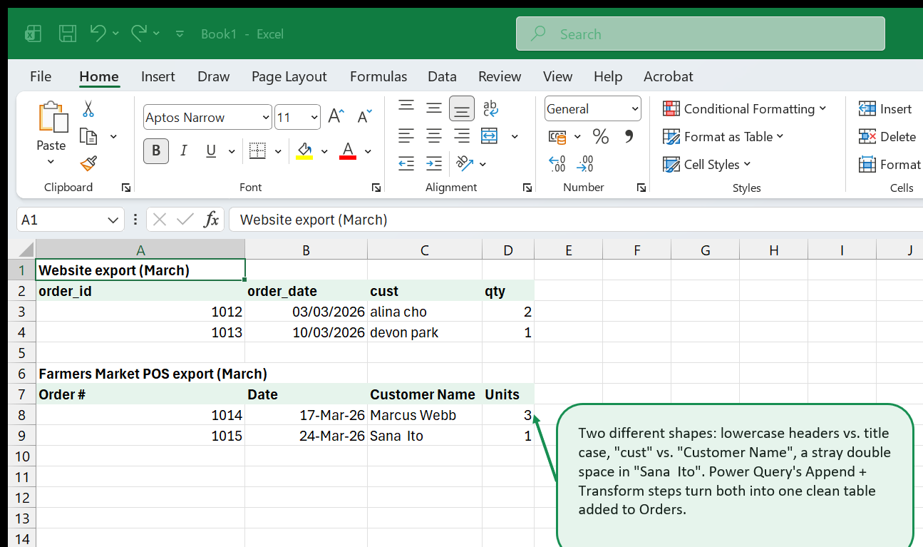
The shape of the fix, click by click: select the website export’s range, Data tab > From Table/Range (Get & Transform group) - this opens the Power Query Editor with that range loaded as a query. Rename its columns to match Orders (right-click a column header > Rename), and use Transform > Format to fix capitalization inconsistencies. Repeat for the POS export as a second query. Then, with both queries open, Append Queries (Home tab, in the Editor) stacks them into one combined table with matching columns. Close & Load To sends the result into the workbook as a new Table, ready to copy into Orders.

The genuinely useful part isn’t this month’s cleanup - it’s that Power Query remembers every step you clicked through, as a named list in the Applied Steps pane. Next month, point the same query at the new export and click Refresh: every rename, every format fix, every append happens again automatically, in seconds, on data that didn’t exist yet when you built the query.

10. Your First Macro: Recording and Running Simple Automation

After this chapter you’ll be able to: record a macro for a repetitive action, assign it to a button, and know what to check when a recorded macro doesn’t behave the way you expected.

A macro is a recorded (or written) sequence of Excel actions, saved under a name, that can be replayed with one click. You don’t need to learn to write VBA code from scratch to get real value from macros - recording one is often enough.

First, turn on the Developer tab if it isn’t visible: File > Options > Customize Ribbon, check “Developer” in the right-hand list. From there, Record Macro starts capturing every action you take until you click Stop Recording. Reyes Roastery’s New Order Entry form (built fully in the next chapter) needs a quick way to blank itself out between orders - clear the SKU, Qty, and any leftover values - so Dana isn’t manually deleting four cells’ worth of content between every sale.

Recording that “clear the form” action on a small selection produces VBA code close to this:

Sub ResetOrderForm()
    Range("B3").ClearContents
    Range("B5").ClearContents
    Range("B3").Select
End Sub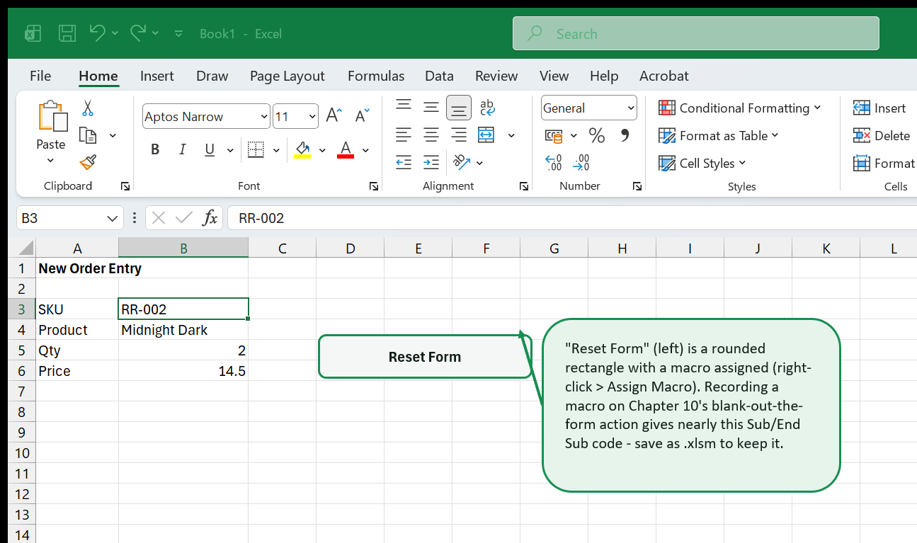

Right-click the shape, choose Assign Macro, and pick ResetOrderForm from the list - clicking the button now runs exactly what was recorded, with no code to write by hand. Relative vs. absolute recording matters here: the default (absolute) always clears the same two cells no matter where the selection started; switching Developer > Use Relative References before recording instead repeats the same relative movement from wherever you begin, useful for a macro meant to act on “the row you’re currently on” rather than one fixed spot.

11. Workbook Automation Basics: Buttons, Events, and a Simple Entry Form

After this chapter you’ll be able to: build a small entry form that fills itself in as you type, using a worksheet event instead of a button click.

Chapter 10’s macro ran when a button was clicked - a command the user triggers on purpose. A Worksheet_Change event macro is different: it runs automatically the instant a specific cell changes, with no button involved at all. Reyes Roastery’s New Order Entry form uses one to auto-fill Product and Price the moment a SKU is chosen from its dropdown.

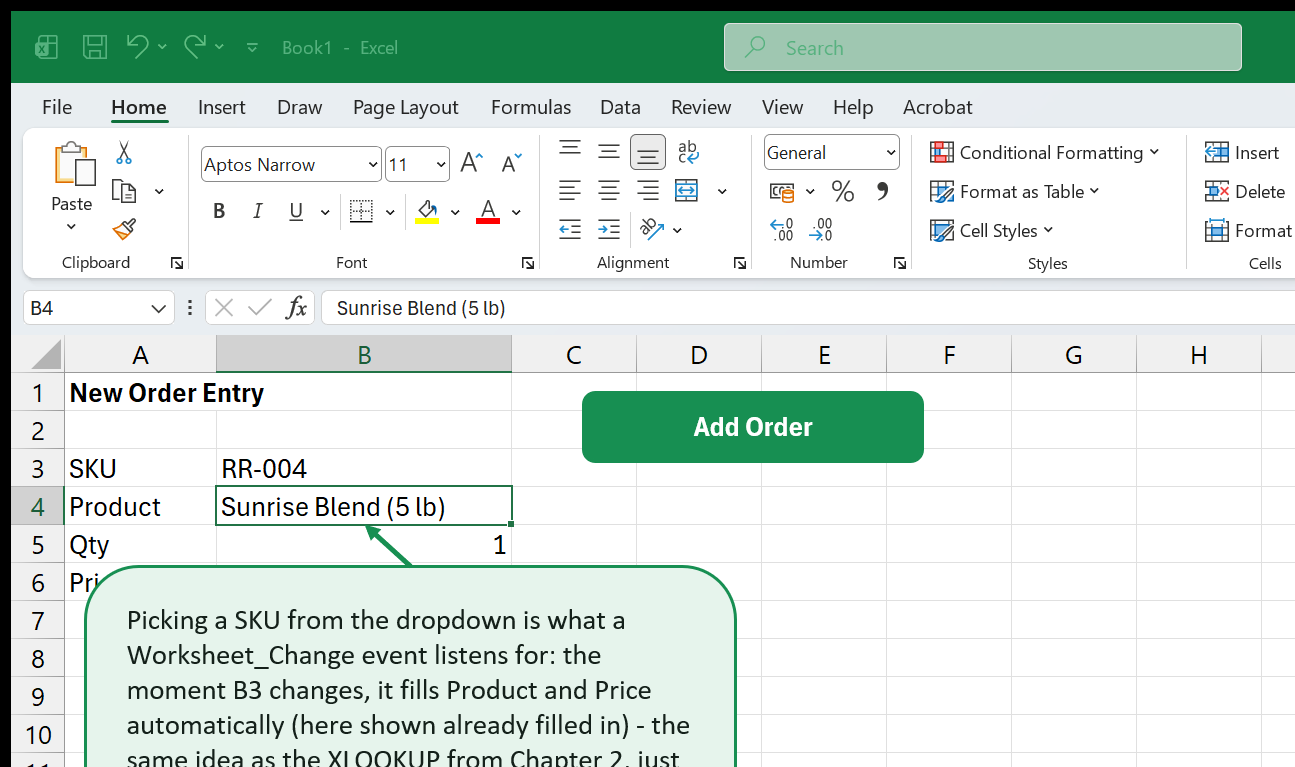
The event lives in the worksheet’s own code module (right-click the sheet tab > View Code), not a general module like Chapter 10’s recorded macro:

Private Sub Worksheet_Change(ByVal Target As Range)
    If Target.Address = "$B$3" Then
        Application.EnableEvents = False
        Range("B4").Value = Application.WorksheetFunction _
            .XLookup(Range("B3").Value, Range("Products[SKU]"), Range("Products[Product]"))
        Range("B6").Value = Application.WorksheetFunction _
            .XLookup(Range("B3").Value, Range("Products[SKU]"), Range("Products[Price]"))
        Application.EnableEvents = True
    End If
End Sub

The Application.EnableEvents = False line is not optional. Without it, this macro’s own change to B4 and B6 would immediately re-trigger Worksheet_Change again, which changes B4/B6 again, which triggers the event again - an infinite loop that freezes Excel. Turn events back on immediately after your own changes are done, in every code path, or a genuine future edit to the sheet stops triggering anything at all.

An “Add Order” button, built the same way as Chapter 10’s Reset Form button, copies the completed form’s four values onto the next blank row of the Orders table with one more short macro - together, choosing a SKU and clicking one button is now the entire process for logging a sale, down from typing five separate values by hand.

PART IV

Where to Go Next

One closing chapter - no new formulas, just the bridge from this book back into the rest of the site, and a certificate worth keeping.

1. Where to Go Next

12. Where to Go Next

Reyes Roastery’s workbook now does, for real, everything this book set out to show: a Table-based product catalog, XLOOKUP-driven order entry, validated dropdowns, a named discount rate, dynamic-array formulas, multi-criteria totals, a grouped-and-sliced PivotTable, a live dashboard, a Power Query cleanup step, and a macro-driven entry form. That’s a genuinely different spreadsheet than the one this book opened with - and the skills behind it transfer directly to whatever you’re actually tracking, coffee or not.

A few places worth going deeper, matched to what this book only had room to introduce:

• The Power Query topic covers query steps, merges, and unpivoting in more depth than one chapter here could - the natural next stop after Chapter 9.
• The PivotTables topic and the PivotTable practice dataset give you more rows to group, slice, and refresh than Reyes Roastery’s small order log.
• The Dashboards & Reporting topic goes further into report layout and design than Chapter 8’s single sheet.
• The Macros & VBA topic has a full article series - the VBA editor, loops and conditions, worksheet events, a common-snippets reference, and error handling - picking up exactly where Chapters 10-11 left off.
• Look up any function from this book - XLOOKUP, FILTER, SORT, UNIQUE, SUMIFS, LET - in the function reference for more worked examples than one book can hold.
• The inventory tracker template is a ready-made starting point if you’d rather adapt a finished workbook than build Reyes Roastery’s from scratch.

Appendix A, next, holds the answer key for every chapter’s self-check quiz - work through them honestly before checking, they’re a genuinely useful signal of what’s actually stuck versus what only looked familiar while reading. After that: your completion checklist.

Appendix A: Self-Check Answers

Chapter 1

1. A workbook is the whole file; a worksheet is one tab inside it. A Table’s name is defined at the workbook level, so any sheet’s formula can reference it (e.g. Products[Price]) without knowing which sheet it physically lives on.
2. A Table gives the range a name usable in formulas, auto-extends formulas and formatting to new rows automatically, and adds sort/filter dropdowns with no extra setup.
3. False - once a range is a Table, use a structured reference like Products[Price] instead, which adjusts automatically as rows are added or removed.

Chapter 2

1. Because the return array ($K$2:$L$6) is two columns wide, so XLOOKUP’s result is a one-row-by-two-column array that spills across two cells instead of one.
2. MATCH finds where the lookup value sits inside a range; INDEX then returns the value at that position - together they do what one XLOOKUP does, in Excel versions that don’t have XLOOKUP.
3. An absolute reference ($J$2:$J$6) stays locked to the same lookup range for every copied row; a relative reference (J2:J6) would shift down with the formula and quickly point at the wrong cells.

Chapter 3

1. Data tab > Data Validation > Allow: List, then either type the valid values directly or point at a range that holds them.
2. Excel rejects the entry and shows a “Stop” alert by default, so the invalid value is never actually entered into the cell.
3. Validating at entry prevents bad data from ever reaching the sheet, which is cheaper and safer than detecting and fixing it after the fact across potentially many rows later.

Chapter 4

1. Select the cell, then Formulas > Define Name - or type the name directly into the Name Box (above the grid, left of the Formula Bar) and press Enter.
2. (1-CaseDiscount) reads in plain English what the formula does; (1-$G$2) requires checking what G2 actually holds. If the named cell is ever moved, every formula using the name keeps working without being edited individually.
3. False - a name can refer to a range of any size, a typed formula, or a constant value, not only a single cell.

Chapter 5

1. It means one formula, entered in a single cell, automatically fills as many neighboring cells as its result needs - without being copied or dragged.
2. It references an entire spilled array from one anchor cell, e.g. =COUNTA(K3#) counts every cell of a spill without hardcoding how many rows it turned out to have.
3. UNIQUE alone returns results in first-seen order; wrapping it in SORT(...) alphabetizes (or numerically orders) the same list.

Chapter 6

1. SUMIF supports exactly one condition; SUMIFS supports multiple conditions and lists the sum range as its first argument (the opposite order from SUMIF).
2. Excel matches each criteria range to the sum range row by row; ranges of different sizes can’t be lined up that way, which triggers a #VALUE! error or an incorrect result.
3. COUNTIFS counts matching rows; SUMIFS totals a numeric column across those same rows - they’d differ whenever any matching row’s summed value isn’t exactly 1 (for example, summing a Qty column where some orders have more than one bag).

Chapter 7

1. It nests inside the first field, grouping and subtotaling within each group of the first field rather than replacing it.
2. A slicer shows every possible value as a clickable button at a glance; a filter dropdown hides the same options behind a menu you have to open first.
3. A PivotTable is built from a cache (a snapshot) of the source data at the time it was created or last refreshed - it does not watch the source range for new rows on its own. Refresh (right-click > Refresh, or Data > Refresh All) re-reads the source and updates it.

Chapter 8

1. The formula stays live - as new orders are added to the source table, the KPI’s number updates automatically instead of slowly going stale like a typed-in figure would.
2. A data bar draws an in-cell bar sized to each row’s value, like a tiny bar chart inside the cell; a color scale shades the whole cell’s fill by its value instead, with no bar shape.
3. The chart would update on its own, since it’s built from a formula-driven range (SUMPRODUCT against the Orders table) that recalculates automatically - not from numbers typed in by hand.

Chapter 9

1. Different column names and casing (order_id vs. Order #, cust vs. Customer Name) and inconsistent formatting (a stray double space inside “Sana Ito”).
2. It combines two or more queries that share a matching column structure into one stacked table.
3. Once a query’s cleaning steps are recorded, Refresh re-runs those exact steps against whatever new data has landed - it doesn’t require redoing the manual cleanup by hand every month.

Chapter 10

1. It gives you access to Record Macro, the VBA editor, and form/ActiveX controls - none of which are on the ribbon by default.
2. Absolute recording (the default) always acts on the exact same cells no matter where the selection started; relative recording repeats the same relative movement from wherever the selection begins when the macro runs.
3. The .xlsx file format has no support for VBA code at all - Excel strips any macro out silently on save, so the file must be saved as .xlsm to keep it.

Chapter 11

1. Any edit to a cell inside the range the macro is written to check - it fires the instant that cell’s value actually changes.
2. Without it, the macro’s own change to other cells would immediately re-trigger Worksheet_Change again, which would trigger it again, in an infinite loop that freezes Excel.
3. Assign the macro to a shape or button (right-click the shape > Assign Macro) so clicking it runs the macro directly, with no VBA editor involved.