INDEX & MATCH Deep Dive

INDEX and MATCH are two of Excel’s most versatile lookup tools — and together they form a combination that outperforms VLOOKUP in almost every practical scenario. Where VLOOKUP is constrained to searching the leftmost column and returning a value to its right, INDEX/MATCH can look in any direction, handle multiple criteria, select columns dynamically, and return the Nth match in a list. If you have used VLOOKUP for years and hit its limits, this guide is for you.

This ebook covers each function individually before combining them. You will see the mechanics clearly: INDEX retrieves a value at a given position, MATCH finds the position of a value in a list. When you nest one inside the other, the result is a flexible lookup engine that works on any data layout. All formulas are shown with realistic examples so you can adapt them directly to your own spreadsheets.

Work through the sections in order the first time, then use the Quick Reference at the end as a daily cheat sheet. Where relevant, comparisons with XLOOKUP are included so you can choose the right tool for each situation. Formulas in this guide assume modern Excel (Microsoft 365 or Excel 2019+) unless otherwise noted.

---

Why INDEX/MATCH, Not Just VLOOKUP

VLOOKUP has a fundamental constraint baked into its design: the lookup column must be the leftmost column in your range, and you return a column to its right by number. That column number is hardcoded, which means inserting or deleting a column silently breaks your formula. It also means VLOOKUP cannot search right-to-left, and it returns only the first match it finds.

INDEX/MATCH has none of those constraints. The lookup column and return column are independent ranges — they do not have to be adjacent, they do not have to be in any particular order, and adding columns to your sheet never breaks the formula. This combination also unlocks two-way lookups, multi-criteria matching, and dynamic column selection with no extra effort.

Capability	VLOOKUP	INDEX/MATCH
Left lookup (return column is left of search column)	No	Yes
Hardcoded column number	Yes	No
Two-way lookup	No	Yes
Multi-criteria match	Workaround required	Yes
Breaks when columns are inserted	Yes	No
Available in all Excel versions	Yes	Yes

The trade-off is verbosity. VLOOKUP is shorter to type. But for anything beyond a simple right-side lookup, INDEX/MATCH is the better investment.

---

How INDEX Works

INDEX returns the value at a specific position inside a range. Think of it as a coordinate system: you supply the range, then tell Excel which row and column to retrieve.

Single-Cell Mode

The most common form takes three arguments: the range, a row number, and an optional column number.

This returns the value in the fifth row of the range C2:C100. If you omit the column number when your range is a single column, Excel assumes column 1.

This returns the value at row 5, column 2 of the range B2:D100 — that is, cell C6 on the sheet.

Range Mode

INDEX can also return an entire row or column by passing zero for one of the position arguments.

Passing 0 for the column number returns every column in row 5 of the range. This is rarely used on its own but becomes useful inside other functions.

Multiple-Area Mode

INDEX accepts a fourth argument, area_num, when you supply multiple non-contiguous ranges separated by commas inside parentheses. This advanced form is uncommon in day-to-day work.

This returns row 3, column 2 from the second area (A8:C12). Stick to single-area mode until you have a specific reason to use this form.

---

How MATCH Works

MATCH finds the relative position of a value within a single row or column and returns a number. It does not return the value itself — just the position. That number is what you feed into INDEX.

The syntax is =MATCH(lookup_value, lookup_array, match_type).

Exact Match (match_type 0)

Use 0 for exact matching. This is the form you will use most often.

This returns 4, meaning “East” is in the fourth row of A2:A100. If the value is not found, MATCH returns a #N/A error.

Approximate Match (match_type 1 and -1)

Match type 1 finds the largest value less than or equal to the lookup value. The array must be sorted ascending. Match type -1 finds the smallest value greater than or equal to the lookup value; the array must be sorted descending.

This is useful for tax bracket lookups, grade scales, and any tiered classification.

Wildcard Match

With match_type 0 you can use * (any characters) and ? (single character) as wildcards.

This matches the first cell in A2:A100 that begins with “East” — such as “East Region” or “Eastern Division”. Wildcard matching is case-insensitive.

match_type	Behavior	Array must be sorted?
0	Exact match	No
1	Largest value <= lookup_value	Ascending
-1	Smallest value >= lookup_value	Descending

---

Combining Them: Your First INDEX/MATCH

The pattern is simple: use MATCH to find the row number, then pass that number into INDEX to retrieve the value.

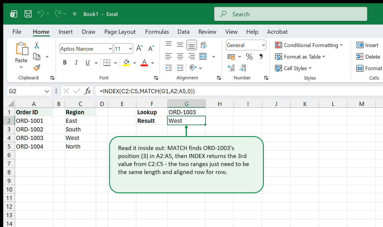
Read it from the inside out. MATCH looks for the value in F1 within A2:A100 and returns a position number. INDEX then uses that position to pull the corresponding value from C2:C100. The two ranges must be the same length and aligned row-for-row.

A concrete example: you have order IDs in column A and regions in column C. Cell F1 contains an order ID. The formula finds the matching row in column A and returns the region from column C for that row.

Making It Robust with IFERROR

Wrap the whole formula in IFERROR to handle cases where the lookup value does not exist.

This returns “Not found” instead of a #N/A error when the value in F1 is not in column A.

---

Left Lookups — Searching Right-to-Left

This is the most common reason people switch from VLOOKUP to INDEX/MATCH. VLOOKUP cannot return a value from a column to the left of the search column. INDEX/MATCH has no such restriction because the lookup range and return range are completely independent.

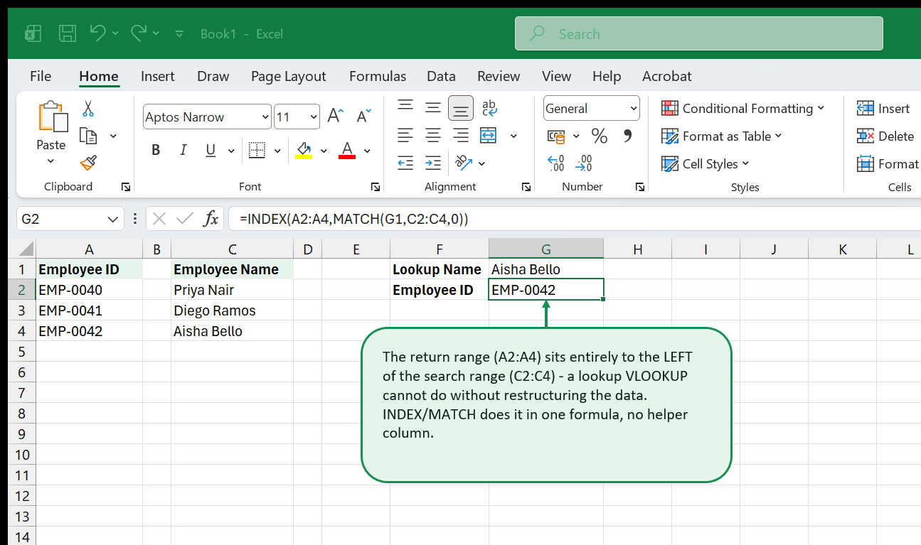
Suppose your data has employee names in column C and employee IDs in column A. You want to look up a name and return the ID — a right-to-left lookup.

The return range (A2:A100) is entirely to the left of the search range (C2:C100). VLOOKUP cannot do this without restructuring your data or adding a helper column. INDEX/MATCH does it in one formula.

---

Two-Way Lookups: Row and Column Together

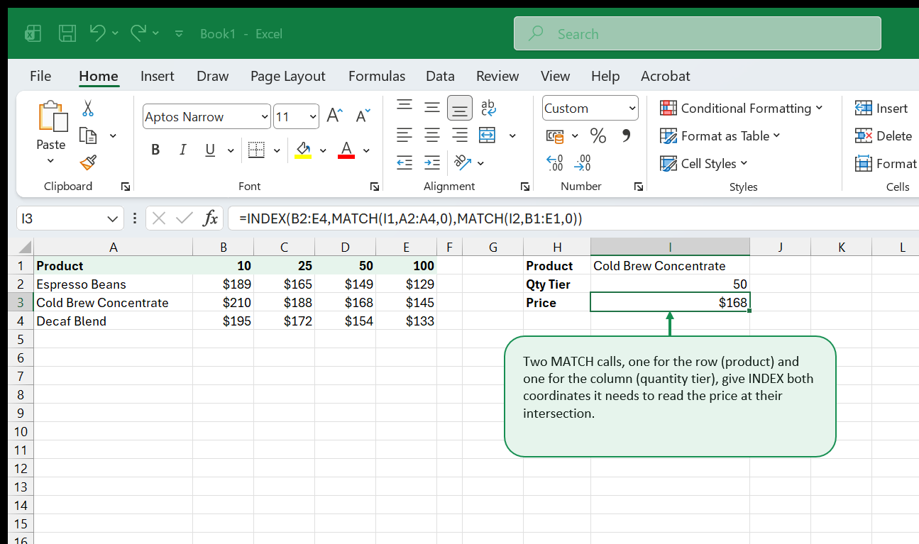
A two-way lookup retrieves a value at the intersection of a matching row and a matching column. This is useful for reading from a matrix — for example, a price table where rows are products and columns are quantity tiers.

The pattern nests two MATCH calls inside INDEX: one for the row position and one for the column position.

Here H1 contains the row lookup value (a product name) and H2 contains the column lookup value (a quantity tier). The first MATCH finds the row, the second finds the column, and INDEX returns the value at their intersection.

Keep the header ranges precise. The row MATCH range (A2:A10) must match the row dimension of the INDEX range (B2:E10), and the column MATCH range (B1:E1) must match the column dimension.

---

Multi-Criteria Lookups with Array Entry

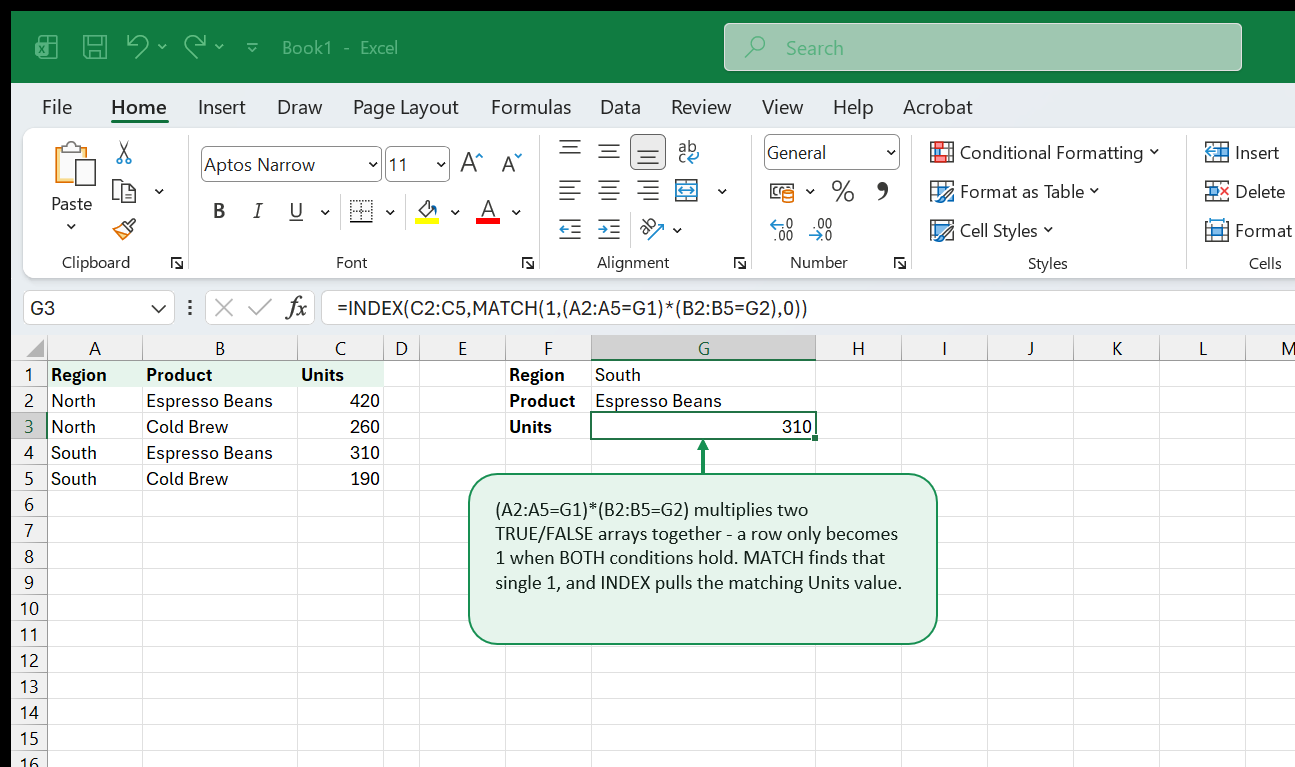
Sometimes you need to match on two or more columns simultaneously — for example, finding a value where both the region and the product match. INDEX/MATCH handles this with an array formula that multiplies two or more conditions together.

In Excel 365 / Excel 2019 (dynamic arrays)

Enter the formula normally with Enter. Excel evaluates the Boolean array automatically.

The inner expression (A2:A100=G1)*(B2:B100=G2) produces an array of 1s and 0s. A row gets 1 only when both conditions are true. MATCH then finds the first 1 in that array, and INDEX retrieves the corresponding value from D2:D100.

In Excel 2016 and Earlier

Press Ctrl+Shift+Enter instead of just Enter. Excel wraps the formula in curly braces { } to indicate array entry. Do not type the curly braces manually.

{=INDEX(D2:D100,MATCH(1,(A2:A100=G1)*(B2:B100=G2),0))}

You can extend this pattern to three or more criteria by adding more multiplication terms.

Each additional criterion narrows the match further. If no row satisfies all criteria, MATCH returns #N/A — wrap in IFERROR to handle this gracefully.

---

Dynamic Column Selection (No Hardcoded Column Numbers)

VLOOKUP requires you to hardcode a column number, such as the third column in the range. When someone inserts a column, that number is wrong and the formula silently returns incorrect data. INDEX/MATCH sidesteps this entirely by using column names from a header row.

Instead of writing INDEX(A:D,row,3), look up the column header dynamically.

G1 holds the row lookup value and H1 holds the column header name you want. The second MATCH finds the column position by name. Now you can insert, delete, or reorder columns and this formula continues to work correctly as long as the header names remain unchanged.

This pattern also enables user-driven column selection. Put a dropdown list of header names in H1 and the formula automatically returns the right column based on whatever the user selects.

---

Returning the Nth Match

VLOOKUP and XLOOKUP both return the first match. INDEX/MATCH can return the second, third, or any specific occurrence of a value with a small extension using SMALL and IF.

In Excel 365 (FILTER + INDEX approach)

Use FILTER to isolate all matching rows and INDEX to pick the Nth one.

G1 is the lookup value and G2 is the occurrence number. FILTER returns all matching values; INDEX picks the one at position G2.

In Excel 2016 and Earlier (SMALL + IF array formula)

{=INDEX(B2:B100,SMALL(IF(A2:A100=G1,ROW(A2:A100)-ROW(A2)+1),G2))}

Enter with Ctrl+Shift+Enter. IF builds an array of row positions where A2:A100 equals G1. SMALL picks the Nth smallest position (Nth match). INDEX retrieves the value at that position.

This formula is verbose but reliable in older Excel versions. In Excel 365, prefer FILTER for clarity.

---

INDEX/MATCH vs. XLOOKUP: When to Use Which

XLOOKUP, introduced in Excel 365 and Excel 2021, handles many cases that previously required INDEX/MATCH. For straightforward lookups, XLOOKUP is shorter and easier to read. But INDEX/MATCH retains advantages in specific situations.

Scenario	Best Tool
Simple vertical lookup, return one column	XLOOKUP
Left lookup	Either (XLOOKUP is simpler)
Two-way lookup	INDEX/MATCH
Multi-criteria with AND logic	INDEX/MATCH (array formula)
Dynamic column selection by header name	INDEX/MATCH
Return Nth match	XLOOKUP with FILTER, or INDEX/MATCH + SMALL
Need to work in Excel 2016 or 2019	INDEX/MATCH
Returning a range (spill behavior)	XLOOKUP

XLOOKUP cannot perform a true two-way lookup in a single formula without nesting another XLOOKUP or MATCH inside it. For matrix intersections, INDEX/MATCH is still the cleaner pattern.

For a detailed comparison of XLOOKUP, VLOOKUP, and the scenarios where each wins, see the XLOOKUP vs VLOOKUP Field Guide.

---

Common Pitfalls

Ranges of Different Lengths

The lookup array in MATCH and the return array in INDEX must have the same number of rows (or columns for a horizontal lookup). If they differ, INDEX returns the wrong value without warning.

=INDEX(C2:C50, MATCH(F1, A2:A100, 0))   ← Wrong: ranges are different lengths
=INDEX(C2:C100, MATCH(F1, A2:A100, 0))  ← Correct

Forgetting match_type 0 for Exact Matches

MATCH defaults to match_type 1 (approximate, sorted ascending) if you omit the third argument. This causes silent incorrect results when your data is not sorted. Always specify 0 for exact matching unless you specifically need approximate behavior.

Extra Spaces and Invisible Characters

If MATCH returns #N/A when you can visually see the value in the list, the most likely cause is leading or trailing spaces. Use TRIM to clean your lookup value.

Number Stored as Text

A number in your data stored as text will not match a true numeric lookup value. Use VALUE() to convert the lookup value, or check the data source. The green triangle in the top-left corner of a cell is Excel’s indicator that a number is stored as text.

Absolute vs. Relative References

When copying INDEX/MATCH across multiple cells, lock the array ranges with dollar signs so they do not shift.

---

Quick Reference

INDEX Syntax

Argument	Description	Example
array	The range to return a value from	C2:C100
row_num	Row position within the array	5
col_num	Column position (optional for single-column ranges)	2

MATCH Syntax

Argument	Description	Example
lookup_value	The value to find	F1
lookup_array	Single row or column to search	A2:A100
match_type	0 = exact, 1 = approx ascending, -1 = approx descending	0

Common Patterns at a Glance

Pattern	Formula Skeleton
Basic lookup	=INDEX(return_range, MATCH(value, search_range, 0))
Left lookup	=INDEX(left_range, MATCH(value, right_range, 0))
Two-way lookup	=INDEX(data, MATCH(row_val, row_range, 0), MATCH(col_val, col_range, 0))
Multi-criteria (365)	=INDEX(return, MATCH(1, (range1=val1)*(range2=val2), 0))
Dynamic column	=INDEX(data, MATCH(row_val, row_range, 0), MATCH(col_header, headers, 0))
With error handling	=IFERROR(INDEX(..., MATCH(...)), "Not found")

Error Troubleshooting

Error	Likely Cause	Fix
#N/A	Value not in lookup array	Check spelling, spaces, data type
#N/A	Wrong match_type	Add 0 as third MATCH argument
#REF!	Row or column number exceeds range size	Check that ranges are the same length
Wrong value returned	Ranges misaligned or different lengths	Make sure ranges start and end on the same rows
Wrong value, no error	match_type omitted, data not sorted	Always specify match_type 0 for exact matches

---

Where to Go Next

INDEX/MATCH becomes even more powerful when combined with Excel’s array and dynamic array features. These guides extend what you have learned here.

• XLOOKUP vs VLOOKUP Field Guide — A direct comparison of the three major lookup functions with decision rules for when to use each.
• Excel Formulas Cheat Sheet — Quick syntax reference for INDEX, MATCH, VLOOKUP, XLOOKUP, FILTER, SORT, and 40+ other functions side by side.
• Explore dynamic array functions (FILTER, UNIQUE, SORT, SORTBY) to handle multi-match scenarios with less formula complexity.
• Practice two-way lookups on a real pricing or scheduling matrix — this pattern appears constantly in financial models and reporting dashboards.
• Once you are comfortable here, study named ranges and structured table references (Table1[Region]) to make INDEX/MATCH formulas even more readable and self-documenting.

Want to practice on a real lookup table instead of the small examples above? Download the VLOOKUP / XLOOKUP practice dataset - a 20-row product lookup table plus a questions sheet, so you can try the same lookups with INDEX/MATCH, VLOOKUP, and XLOOKUP side by side.