Excel for Finance & Accounting

Finance and accounting work lives in Excel. Whether you are preparing a monthly income statement, evaluating a capital investment, or tracking actuals against a budget, spreadsheet fluency is the skill that separates analysts who answer questions quickly from those who are still formatting cells when the meeting starts. This guide is for anyone who already knows basic Excel — you can write a SUM formula and navigate worksheets — and wants to use it confidently for real financial work.

Every example in this guide is built around Reyes Roastery, a small but growing specialty coffee business with two retail locations and a wholesale channel. The numbers are invented, but the problems are real: building a budget, modeling a loan, mapping transactions to account codes, and producing reports that management can actually read. Working through a single consistent scenario means you can see how the pieces fit together rather than learning a collection of disconnected tricks.

Work through the chapters in order the first time. Chapter 1 through Chapter 3 establish the foundation — workbook structure, number formatting, and the time-value functions that underpin almost every financial calculation. Chapters 4 through 9 build the actual models. Chapter 10 covers the practical step that most tutorials skip: locking down the finished file before you share it. If you already have a specific need, jump to that chapter; each section is self-contained enough to stand alone.

Setting Up a Finance-Ready Workbook

A well-structured workbook prevents errors before they happen. The choices you make in the first five minutes — how many sheets, what they are named, where inputs live — determine how easy the file is to audit, extend, and hand off six months from now.

The Sheet Stack

Reyes Roastery’s workbook uses a consistent sheet order that mirrors how data flows from raw inputs to finished reports.

Sheet	Purpose
Assumptions	All input values: prices, rates, headcount, growth targets
Data	Transaction-level detail or monthly actuals pasted from the accounting system
Accounts	Chart of accounts lookup table for categorization
P&L	Income statement summary driven by formulas, never typed values
CashFlow	Indirect cash flow model
Variance	Budget vs. actual comparison with conditional formatting
Dashboard	Key metrics for sharing with non-Excel users

Color-code the tabs. Right-click any sheet tab, choose Tab Color, and assign a consistent scheme: blue for input sheets, green for model sheets, gray for reference tables, orange for outputs. Anyone opening the file immediately understands the structure.

Separating Inputs from Formulas

The single most important workbook design rule: never hard-code a number that might change inside a formula. If the corporate tax rate appears in twenty formulas, you will miss one when it changes. Instead, put the rate in a named cell on the Assumptions sheet and reference that cell everywhere.

To name a cell, select it, click the Name Box at the left of the formula bar, type a name like TaxRate, and press Enter. You can then write:

Named ranges also make formulas readable. =Revenue - COGS - OpEx communicates intent in a way that =B12 - B28 - B41 does not.

Locking the Assumption Range

Select the input cells on the Assumptions sheet and give the range a background color (light yellow works well for conventions many finance teams use). This signals to collaborators that these cells are intentional inputs, not errors to be overwritten. You will formalize this with sheet protection in Chapter 10.

Number Formats That Make Reports Professional

A cell displaying 47832.5 and a cell displaying $47,832.50 contain identical data. The format controls only how the number is presented, never its value. Choosing the right format is fast, free, and makes every report look as though it was built by someone who cares.

The Custom Format String

Excel’s built-in formats cover most needs. For anything else, open the Format Cells dialog (Ctrl+1), go to the Number tab, choose Custom, and type a format code. Finance work uses a handful of patterns repeatedly.

Code	Display	Use
#,##0	47,833	Whole-number counts and quantities
#,##0.00	47,832.50	General currency without symbol
"$"#,##0.00	$47,832.50	Dollar amounts
#,##0.00_);(#,##0.00)	(1,250.00)	Accounting style, negatives in parentheses
0.0%	23.4%	Percentages with one decimal
0.00x	2.35x	Multiples (EV/EBITDA, coverage ratios)
mmm yyyy	Jul 2026	Month-year column headers

Thousands and Millions Scaling

When your model spans millions of dollars, showing every digit clutters the report. A trailing comma in a custom format code divides the displayed value by 1,000.

• #,##0, shows 47,833,000 as 47,833 (thousands)
• #,##0,, shows 47,833,000 as 48 (millions, rounded)
• "$"#,##0,,"M" shows 47,833,000 as $48M

The underlying cell value is unchanged. Formulas that reference the cell use the full precision.

Consistent Sign Conventions

Pick a sign convention and apply it to the entire workbook. The two common choices:

• Revenue positive, costs positive: EBITDA = Revenue - Costs. Simple arithmetic, but subtraction is explicit.
• Costs negative: EBITDA = SUM(Revenue:Costs). Every line just adds up. This is the convention used in this guide and in most professional models.

Whichever you choose, document it in a cell on the Assumptions sheet.

Time Value of Money: PV, FV, and PMT

The three core time-value functions — PV, FV, and PMT — appear in every kind of financial analysis from lease evaluations to retirement projections. Understanding them deeply is more valuable than memorizing their syntax.

PMT: Calculating a Loan Payment

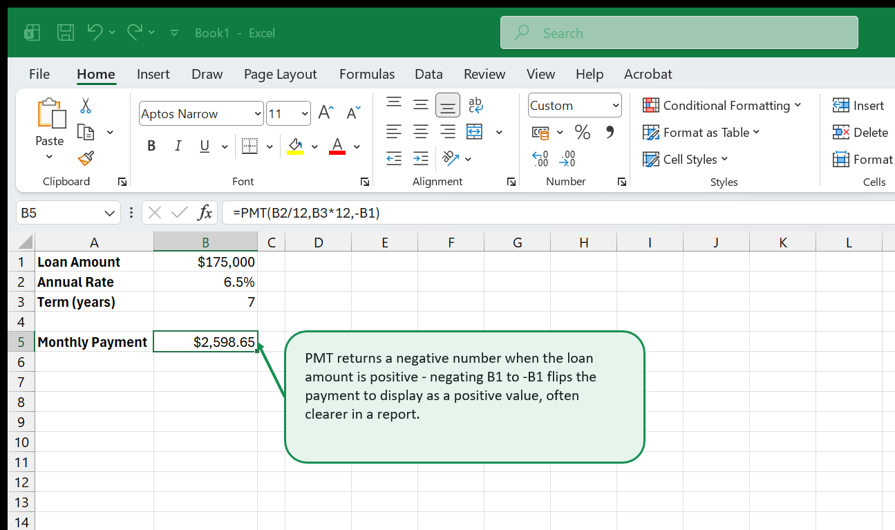
Reyes Roastery is evaluating a $175,000 equipment loan at 6.5% annual interest over seven years. The monthly payment is:

Cell	Label	Value
B2	Loan Amount	175,000
B3	Annual Rate	6.5%
B4	Term (years)	7

Note the sign: PMT returns a negative number when the present value is positive (cash received). Negating the loan amount as -B2 makes the payment display as positive, which is often clearer in a report. The /12 and *12 convert the annual rate and year count to monthly periods — PMT requires that rate and nper always use the same period.

PV: What Is a Future Stream Worth Today?

The roastery is evaluating a wholesale contract that pays $4,000 per month for five years. Using an 8% discount rate, the present value of that stream is:

If the upfront cost to acquire the contract (new equipment, setup) exceeds $197,932, the deal destroys value at this discount rate.

FV: Projecting Savings Growth

If the roastery sets aside $2,500 per month in a reserve account earning 4.2% annually, after three years the balance will be:

The zero for the fourth argument (pv) means there is no existing balance. Changing that argument lets you project growth for an account that already has funds.

RATE and NPER

Two less-used but equally important functions complete the set. RATE finds the interest rate implied by known payment, term, and amount:

NPER finds how many periods a payment takes to retire a balance:

Both use the same sign convention rules as PMT.

NPV and IRR for Investment Decisions

Loan math answers “how much does this cost?” Investment analysis asks the harder question: “is this worth doing?” NPV and IRR are the standard tools for that question.

Setting Up a Cash Flow Timeline

Before writing a single formula, build a cash flow timeline in a column. Reyes Roastery is considering opening a third location. The analysis lives on its own sheet with one row per year, Year 0 through Year 5.

Row	Year	Cash Flow	Notes
5	0	(185,000)	Initial investment
6	1	28,000	Ramp-up year
7	2	54,000
8	3	71,000
9	4	78,000
10	5	82,000

NPV: Net Present Value

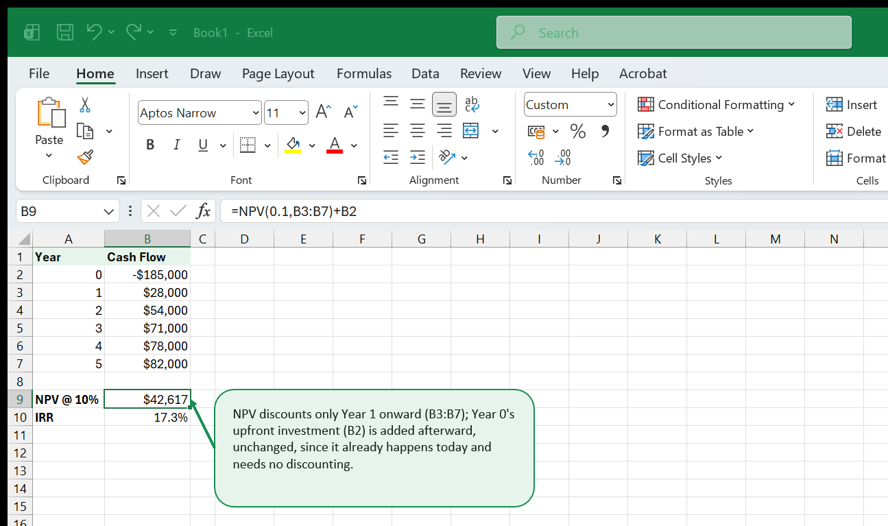
NPV discounts future cash flows back to today at a chosen rate and sums them. It does not include Year 0 automatically — you add that separately.

A positive NPV means the project returns more than the cost of capital. At a 10% discount rate, this location adds $41,847 of value in today’s dollars.

A common mistake: wrapping all cash flows including Year 0 inside NPV. The function treats the first value in the range as occurring at the end of Period 1, so including Year 0 inside it discounts a cash flow that should not be discounted at all.

IRR: Internal Rate of Return

IRR finds the discount rate at which NPV equals zero. It is the project’s implied annual return.

If the company’s required return (hurdle rate) is 10%, a project returning 21.3% clears the bar. Report both NPV and IRR together — IRR alone can mislead when projects differ in scale or have unusual cash flow patterns.

Sensitivity with a Data Table

After calculating base-case NPV, build a one-variable data table to show NPV across a range of discount rates. In a column below the model, list rates from 5% to 25% in 1% increments. In the row above that column, write a formula that references your NPV cell. Select the full range, go to Data tab > What-If Analysis > Data Table, enter your discount rate cell as the Column Input Cell, and click OK. Excel fills in the NPV for each rate automatically.

SUMIFS for Budget vs. Actual Tracking

SUMIFS is the workhorse of management accounting. It lets you slice a transaction table by any combination of criteria — month, account, location, cost center — and pull a subtotal into a summary report.

The Transaction Table

All of Reyes Roastery’s transactions live on the Data sheet as a structured table (Insert > Table) named Transactions. The columns are:

Column	Field
A	Date
B	Location (Downtown, Eastside, Wholesale)
C	Account Code
D	Account Name
E	Amount

Keeping data as a named table means formulas that reference it automatically expand when new rows are added.

Basic SUMIFS

Total revenue for the Downtown location in June 2026:

The date criteria use >= and < with DATE() to bracket a full month without hard-coding text strings. This pattern works for any month — change the year and month numbers in DATE() and the formula recalculates.

Building a 12-Month Budget vs. Actual Matrix

On the Variance sheet, set up a grid with months across columns (B through M) and account lines down rows. In the header row, put the first day of each month: =DATE(2026,1,1) in B1, =EDATE(B1,1) in C1, dragged right to M1. Format the header row as mmm to show abbreviated month names.

In each data cell, SUMIFS pulls actual spend for that account and month:

The mixed references ($A5 locks the column, B$1 locks the row) allow this formula to be copied across the entire grid correctly.

SUMPRODUCT as an Alternative

When criteria involve calculated conditions — for example, filtering by quarter — SUMPRODUCT is more flexible than SUMIFS:

Each parenthetical expression evaluates to an array of 1s and 0s. Multiplying the arrays together acts as AND logic. The result is the sum of amounts where all conditions are true.

Lookup Functions for Account Mapping and Categorization

When transactions come out of an accounting system, they carry account codes but not always account descriptions or grouping categories. Lookup functions translate codes into the labels and categories your P&L needs.

XLOOKUP: The Modern Standard

XLOOKUP replaced VLOOKUP as the preferred lookup function starting with Microsoft 365. It searches a lookup array and returns a value from a return array, without requiring you to count column positions.

The Accounts sheet has code in column A, account name in column B, and reporting category (Revenue / COGS / OpEx / Other) in column C.

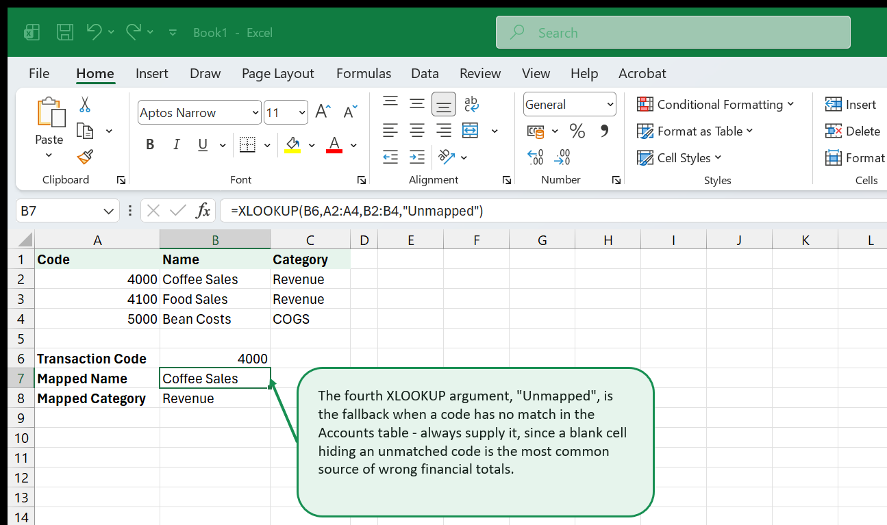
The fourth argument ("Unmapped") is the value to return when no match is found. Always supply it — a blank cell hiding an unmatched code is the most common source of incorrect financial totals.

To pull the category instead of the name, change the return array:

Nested XLOOKUP for Two-Tier Mapping

The roastery uses sub-categories within OpEx (Labor, Occupancy, Marketing, G&A). A second lookup on the sub-category table maps each account to its reporting line:

Inner lookups resolve first. Excel evaluates the inner XLOOKUP to get the sub-category code, then passes that result to the outer XLOOKUP.

Reference Table: Lookup Functions

Function	Syntax	Returns	When to Use
XLOOKUP	XLOOKUP(value, lookup_arr, return_arr, [if_not_found])	Single value or array	Default choice in Microsoft 365
VLOOKUP	VLOOKUP(value, table, col_num, [exact])	Value from nth column	Legacy files, older Excel versions
MATCH	MATCH(value, array, [type])	Position number	When you need the row/column number itself
INDEX	INDEX(array, row, [col])	Value at position	Combined with MATCH for flexible lookups
IFERROR	IFERROR(formula, value_if_error)	Formula result or fallback	Wrapping any lookup to suppress #N/A

Building an Income Statement

With the Data sheet populated and the Accounts sheet mapping codes to categories, the P&L sheet can pull everything together into a formatted income statement driven entirely by formulas.

Structure of the P&L Sheet

The income statement uses a standard waterfall structure. Each section summarizes to a subtotal, and each subtotal feeds the next section.

Revenue
  Coffee Sales
  Food Sales
  Wholesale
  Total Revenue

Cost of Goods Sold
  Total COGS

Gross Profit

Operating Expenses
  Labor
  Occupancy
  Marketing
  G&A
  Total OpEx

EBITDA

Depreciation & Amortization
EBIT

Interest Expense
EBT

Income Tax
Net Income

Each line is a SUMIFS formula pulling from the Transactions table, filtered to the period shown in the header row and to the relevant account codes.

Year-to-Date vs. Period Columns

Set up the column structure to show both monthly and year-to-date figures side by side. For a June 2026 report:

Column	Header	Formula Type
B	Jun 2026 Actual	SUMIFS for June dates only
C	Jun 2026 Budget	Reference to Budget sheet
D	Jun Variance	=B - C
E	YTD Actual	SUMIFS for Jan 1 through Jun 30
F	YTD Budget	Sum of budget columns Jan through Jun
G	YTD Variance	=E - F

Gross Margin and EBITDA Margin

Below the main statement, calculate key ratios. Expressing ratios as formulas tied to the statement means they update automatically:

(Replace B_GrossProfit and similar with your actual cell references or named ranges.)

Building a Cash Flow Model

The income statement shows profitability. The cash flow statement shows whether the business has cash to pay its bills. The two can diverge significantly when a business is growing, investing heavily, or managing large receivables balances.

The Indirect Method

The indirect method starts with net income and adjusts for non-cash items and working capital changes. It is the most common format for management reporting because the inputs are already available from the P&L and balance sheet.

The CashFlow sheet references the P&L for its starting point:

Working Capital Adjustments

Each working capital line is the change in the balance from the prior period to the current period. An increase in accounts receivable uses cash (negative adjustment); an increase in accounts payable provides cash (positive adjustment).

Line	Formula	Logic
Change in Receivables	=-(B_AR - A_AR)	Increase = cash used
Change in Inventory	=-(B_Inv - A_Inv)	Increase = cash used
Change in Payables	=B_AP - A_AP	Increase = cash provided
Change in Accrued Liabilities	=B_Accr - A_Accr	Increase = cash provided

The B_ and A_ prefixes reference current-period and prior-period balance sheet cells respectively.

Operating, Investing, and Financing Sections

Structure the model in three labeled sections:

Operating Cash Flow starts with net income, adds back depreciation (non-cash expense), and applies working capital adjustments.

Investing Cash Flow captures capital expenditures and asset disposals. Capex is negative (cash out):

Financing Cash Flow captures debt draws, repayments, and any equity transactions:

Net Change in Cash sums the three sections and should reconcile to the change in the cash balance on the balance sheet — a powerful built-in check:

If this number does not match Ending Cash - Beginning Cash, there is an error somewhere. Build the check explicitly as a formula and flag it with a conditional format that turns red when it is not zero.

Variance Analysis with Conditional Formatting

A variance report becomes actionable when the numbers most deserving of attention are immediately visible. Conditional formatting does that work automatically.

Calculating Variance and Variance Percent

On the Variance sheet, each row has an Actual column, a Budget column, and two calculated columns:

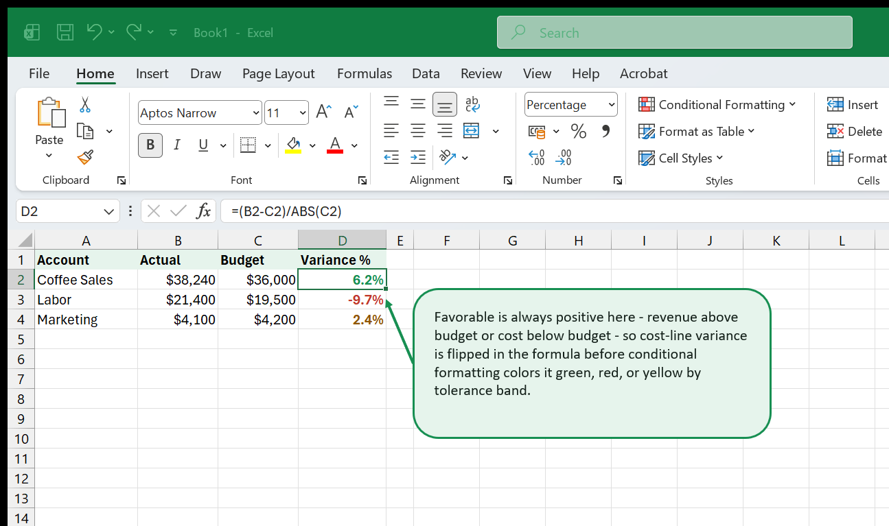
Using ABS(B_Budget) in the denominator handles the case where budget is negative (a cost line) correctly. Variance percentage without ABS can flip signs unexpectedly.

Favorable vs. Unfavorable Convention

In finance reporting, “favorable” means the variance improves profit: revenue above budget (positive) or cost below budget (negative). Build a helper column:

This flips the sign for cost lines so that positive always means favorable. Apply your color rules to this helper column rather than to the raw variance.

Applying Conditional Formatting Rules

Select the Variance % column. On the Home tab, choose Conditional Formatting > New Rule. Use Format only cells that contain to set up three rules, applied in order:

1. Cell value less than -5% → Red fill, white bold text (significant unfavorable)
2. Cell value greater than 5% → Green fill (significant favorable)
3. Cell value between -5% and 5% → Yellow fill (within tolerance)

For a more visual approach, use Data Bars or a 3-Color Scale on the absolute variance column. Data bars show relative magnitude at a glance without requiring the reader to interpret numbers.

Sparklines for Trend Context

A single month’s variance can be misleading — a line might be running unfavorable all year, or last month might be an isolated spike. Insert sparklines to show the 12-month trend in a narrow column next to the variance percentage.

Select the 12-month actual data for the first account row. Go to Insert > Sparklines > Line. Set the Location Range to a single cell in the trend column. Copy the sparkline cell down through all account rows. Format the sparklines to show the high and low points as markers.

Protecting Formulas and Sharing Safely

A finished financial model has two types of cells: inputs that users should change, and formulas that users should not. Mixing them up — overwriting a formula with a typed number — is one of the most common and hardest-to-detect errors in spreadsheet work.

Unlocking Input Cells First

By default, every cell in Excel is locked. Sheet protection respects this lock flag, so locking everything protects formulas but also prevents users from entering inputs. The correct sequence:

1. Select all cells: Ctrl+A
2. Unlock all: Ctrl+1 > Protection tab > uncheck Locked > OK
3. Select only formula cells: Use Ctrl+G > Special > Formulas to select all formula cells at once
4. Re-lock formulas: Ctrl+1 > Protection tab > check Locked > OK

Now all cells are unlocked except the formula cells.

Activating Sheet Protection

Go to Review tab > Protect Sheet. Set a password (store it in your password manager, not in the file itself). Under “Allow all users of this worksheet to:”, check only what you want users to be able to do — typically “Select unlocked cells” is sufficient. Click OK.

Protected formula cells now show an error message if a user tries to edit them, while input cells remain fully editable.

Protecting Multiple Sheets at Once

For a workbook with many sheets, protecting each one individually is tedious. This short macro protects all sheets with a single password:

Sub ProtectAllSheets()
    Dim ws As Worksheet
    Dim pwd As String
    pwd = "ReyesQ3Model"
    For Each ws In ThisWorkbook.Worksheets
        ws.Protect Password:=pwd, DrawingObjects:=True, Contents:=True, Scenarios:=True
    Next ws
    MsgBox "All sheets protected."
End Sub

Open the VBA editor with Alt+F11, insert a Module, paste this code, and run it with F5. Change the password before using in production.

Hiding Formulas from the Formula Bar

For models you share externally, you may also want to hide the formula logic itself. With formula cells selected, go to Format Cells > Protection and check both Locked and Hidden. After sheet protection is applied, the formula bar shows nothing when a protected formula cell is selected — users see the result but cannot reverse-engineer the calculation.

Preparing the File for Distribution

Before sending a model to someone outside your team, run through this checklist:

• Remove any personal data or preliminary figures on hidden sheets (check with Format > Sheet > Unhide to see if any exist)
• Review named ranges (Formulas > Name Manager) and delete any that reference deleted sheets
• Save as .xlsx rather than .xlsm if the workbook contains no macros needed by recipients
• Set the print area and page breaks on each output sheet so the file prints cleanly
• Test the file by opening it on a machine without your linked data sources

Where to Go Next

This guide covered the core financial functions and model-building patterns that appear in most accounting and finance work. The following resources build directly on what you have learned here:

• Excel Formulas Cheat Sheet — a compact reference for every function used in this guide plus the full Excel formula library, organized by category
• Financial Modeling topics — deeper coverage of three-statement models, scenario analysis, and Monte Carlo simulation
• Excel’s built-in template gallery — File > New, search “financial” for income statement, cash flow, and loan amortization templates you can adapt to your own workbook structure
• Microsoft Support: XLOOKUP function — the official documentation covers array returns, approximate match modes, and binary search performance that were not covered here
• Want to build the PMT/EDATE patterns from this guide on real numbers? Download Financial modeling starter: loan amortization - a single-sheet PMT-driven amortization schedule with a month-by-month interest, principal, and balance breakdown.