Excel for Beginners

If you have never opened Excel, or you have used it for years without ever feeling sure you were doing it “right,” this book is for you. It covers the Excel screen, entering and formatting data, how formulas actually work, the handful of functions that cover most real work, and a first look at charts, PivotTables, and cleaning up messy data. Nothing here assumes you already know spreadsheet terms.

Eighteen short chapters, each one buildable in a few minutes. Work through them in order the first time - later chapters lean on earlier ones - then keep the PDF as a reference.

1. What Excel Actually Is (and Isn’t)

Excel is a grid of boxes called cells, arranged into columns (lettered A, B, C…) and rows (numbered 1, 2, 3…). Every cell can hold one of three things: a number, text, or a formula that calculates something from other cells. That’s the entire model. Everything else - formatting, charts, PivotTables, functions - is built on top of those three ideas.

What Excel is good at: anything with numbers that need to be totaled, compared, sorted, or recalculated when an input changes. Budgets, schedules, inventories, simple databases, quick charts. What it is not: a word processor, a design tool, or a real database once you’re past a few tens of thousands of rows with multiple related tables - at that point, tools like Access or a proper database take over, though the vast majority of individual and small-business work never gets there.

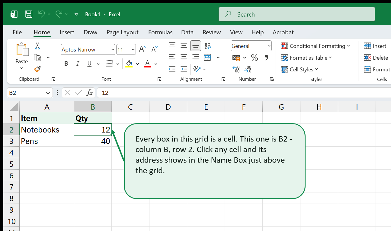
A cell’s address - its column letter plus its row number, like B2 - is called a cell reference. You will see cell references constantly: formulas are built almost entirely out of them. Click any cell right now (in a real workbook, if you have Excel open alongside this book) and look at the box just above the grid, on the left - it shows the address of whatever cell is selected. That box is called the Name Box, and it’s the subject of the next chapter.

One more distinction worth making early: a workbook is the whole file (what you save, email, or download); a worksheet (or just “sheet”) is one page inside that file, shown as a tab along the bottom. A workbook can hold one sheet or dozens.

2. The Excel Screen: Ribbon, Cells, Sheets, and Views

The Excel window has four regions worth naming, because the rest of this book refers to them by name.

• The Ribbon - the row of tabs across the top (Home, Insert, Page Layout, Formulas, Data, Review, View, and more). Each tab groups related commands. Home has the everyday tools: fonts, alignment, number formats, and basic editing. Insert has charts, tables, and PivotTables. Formulas has function tools. Data has sorting, filtering, and Remove Duplicates. You do not need to memorize which tab holds what - you’ll absorb it by using it, and Excel’s own search box (the magnifying glass, usually top right) finds any command by name if you forget.
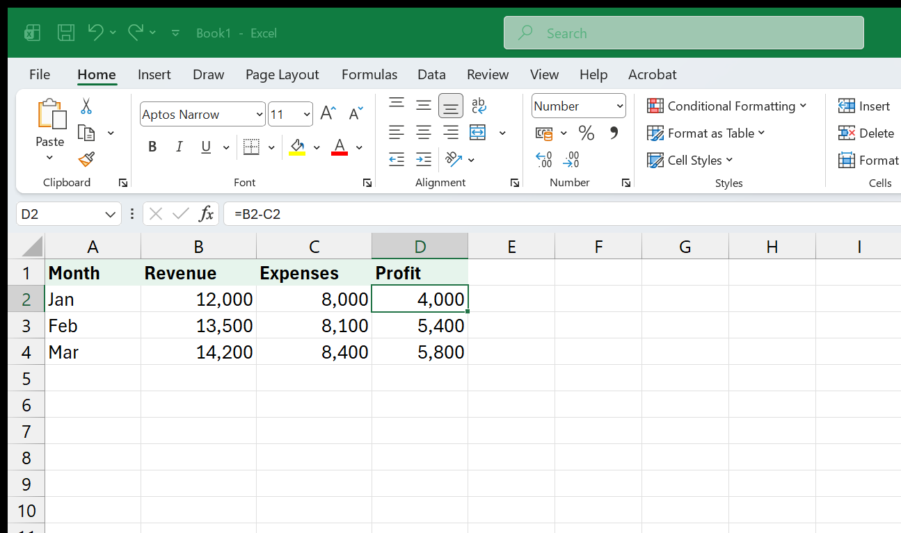
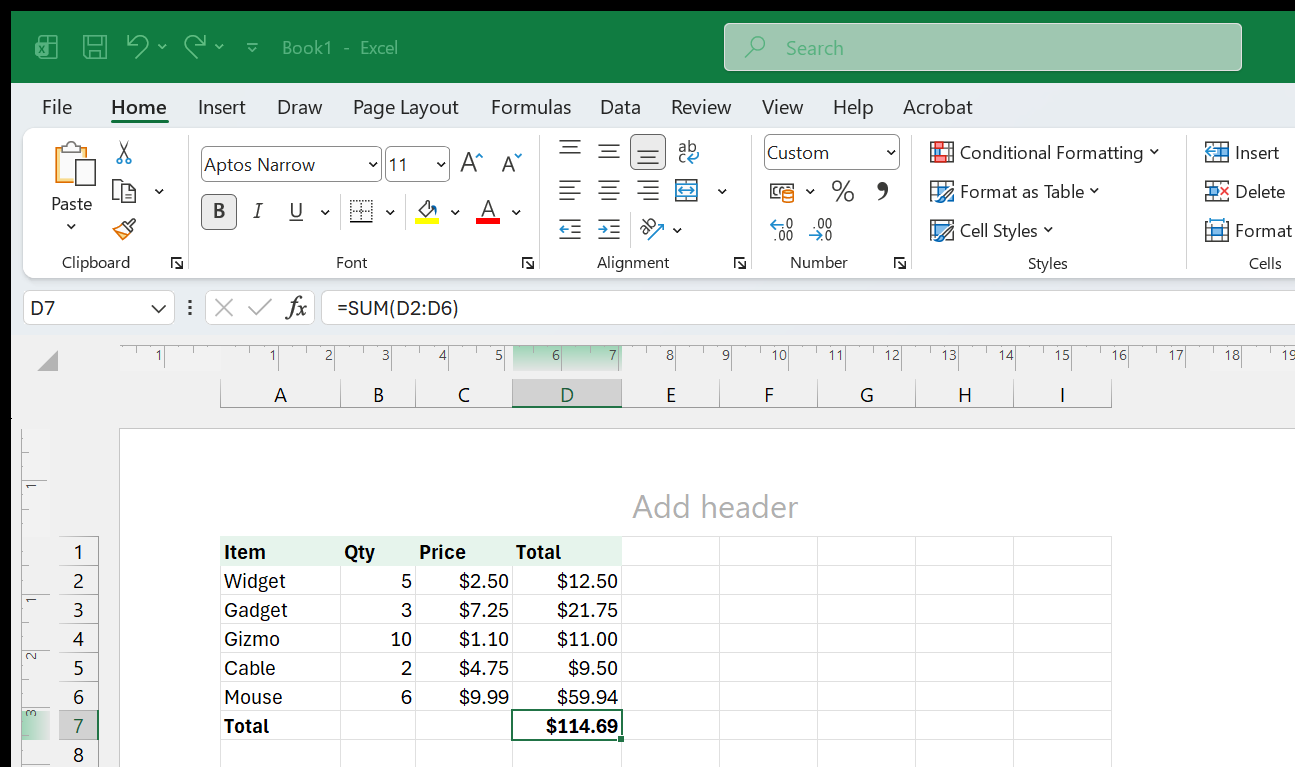
• The Name Box and Formula Bar - directly above the grid. The Name Box (left) shows the address of the selected cell; the Formula Bar (right, the long one) shows that cell’s actual contents - the raw formula, not just the calculated result. This distinction matters constantly: a cell might display $114.69, but the Formula Bar might show =SUM(D2:D6).
• The grid - rows and columns of cells, with gray column letters and row numbers along the edges (the “headers,” not to be confused with a table’s own header row of labels).
• Sheet tabs - along the bottom, one per worksheet in the workbook. A workbook can have any number of sheets; right-click a tab to rename, color, add, or delete one.

Excel also has a handful of views, switched from the View tab or the three small icons in the bottom-right corner of the window: Normal (the default, for data entry), Page Layout (shows exactly how the sheet will print, margins included - covered in Chapter 7), and Page Break Preview (for adjusting where pages split). Most day-to-day work happens in Normal view; you’ll only reach for the others when formatting or printing.

3. Opening, Saving, and Navigating Workbooks

Excel’s default file format is .xlsx. Older files (from Excel 2003 and earlier) use .xls; if you ever see “Compatibility Mode” in the title bar, you’re working in one of those and some newer features may be unavailable until you save as .xlsx.

Saving. Ctrl+S saves the current file. The first time you save a new workbook, Excel asks where. After that, Ctrl+S saves silently to the same location - get in the habit of pressing it often, not just when you’re done. Ctrl+Shift+S (or File > Save As) saves a new copy under a different name or location, leaving the original untouched - useful before a risky edit, or when you want to keep a dated backup of a workbook you update regularly.

Opening. Ctrl+O opens the Open dialog. Excel also keeps a “Recent” list (File > Open > Recent) of files you’ve worked in lately, which is usually faster than browsing folders.

Navigating within a workbook. Ctrl+Page Down / Ctrl+Page Up moves one sheet tab to the right or left - faster than clicking tabs once you have more than a few. Within a sheet, Ctrl+Arrow (any direction) jumps to the edge of the current block of data, and Ctrl+Home always returns you to cell A1. These four shortcuts alone cover most of the moving-around you will ever need to do by keyboard, and they’re worth learning before the fuller shortcut list in Chapter 18.

AutoSave, if you see it in the title bar (only available when a file is stored in OneDrive or SharePoint), saves continuously in the background - useful, but it also means “undo my last hour of changes by closing without saving” is no longer an option the way it was with a purely local file. Know which mode you’re in before you rely on either behavior.

4. Entering and Editing Data

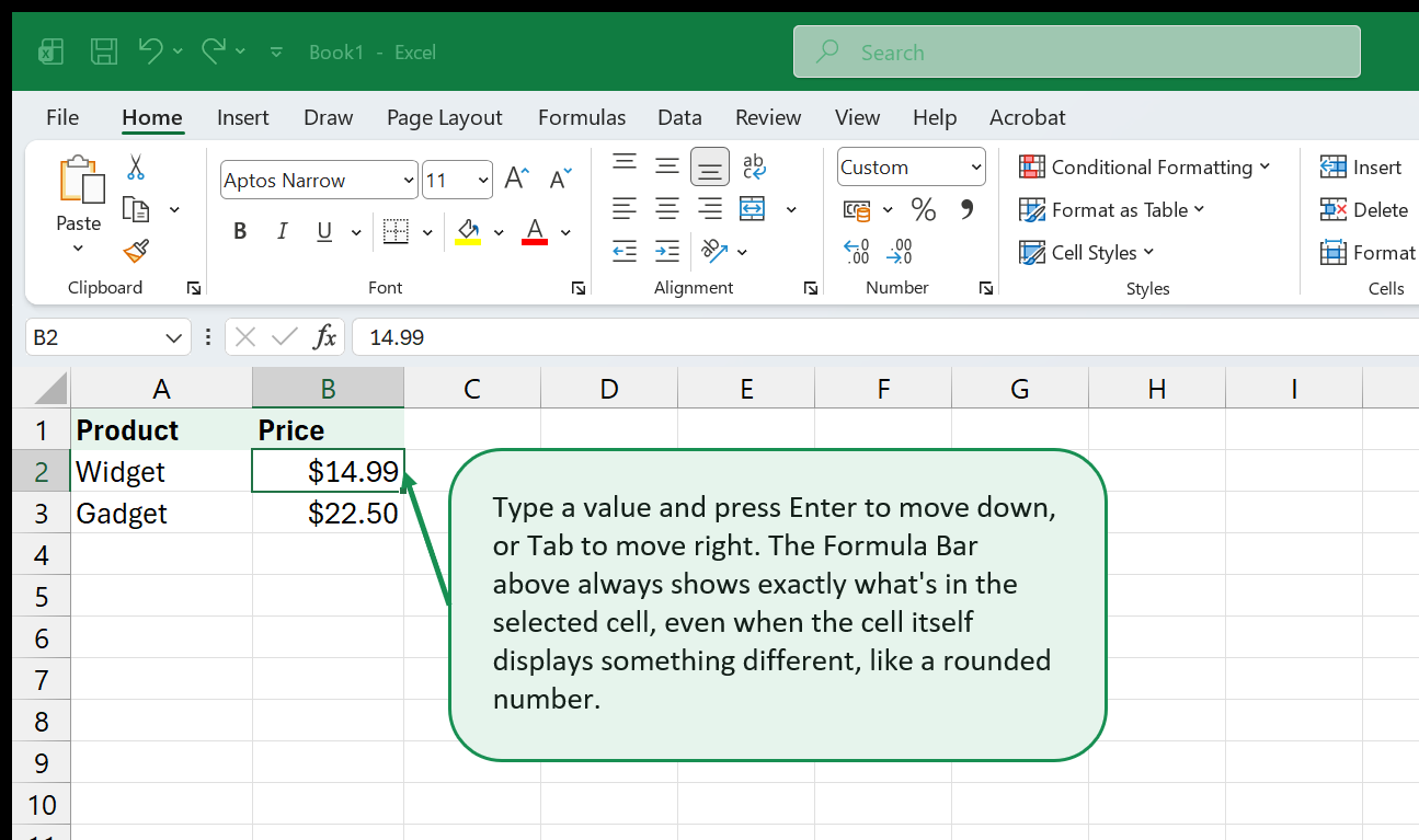
Click a cell, type, and press Enter (moves down) or Tab (moves right) to confirm. Esc cancels an edit in progress without changing the cell. Double-click a cell (or press F2) to edit its existing contents in place, rather than replacing them.

A few habits worth building early:

• Numbers are numbers, text is text - Excel decides which on entry. Type 14.99 and it’s a number (right-aligned by default, usable in math). Type Widget and it’s text (left-aligned, not usable in arithmetic). This matters later: a number that got typed with an accidental leading space, or pasted from a system that quoted it, can silently become text - and a text-that-looks-like-a-number breaks SUM and other math functions in ways that are confusing to debug if you don’t know to check for it.
• The fill handle - the small square at the bottom-right corner of a selected cell - lets you drag to copy a value or formula into adjacent cells. Drag it down a column of dates or numbered items (“Jan”, “Feb”… or “1”, “2”…) and Excel extends the pattern automatically; drag it down a formula and Excel adjusts the cell references for each row (this is relative referencing, covered fully in Chapter 9).
• Undo (Ctrl+Z) and Redo (Ctrl+Y) work across almost everything, including formatting and structural changes like inserting rows - not just typed content. If something looks wrong, undo before you assume you need to retype it.
• Copy (Ctrl+C), Cut (Ctrl+X), Paste (Ctrl+V) work as you’d expect, with one detail worth knowing: Paste Special (Ctrl+Alt+V) lets you paste just the value, just the formatting, or just the formula separately - useful when you want a calculated result frozen as a plain number, without the formula that produced it.

5. Formatting Cells: Numbers, Dates, Currency, and Styles

Formatting changes how a value looks, never what it actually is. This is the single most important idea in this chapter: a cell formatted as Currency to show $1,234.50 still holds the number 1234.5 underneath, and any formula that references it uses the real number, not the display.

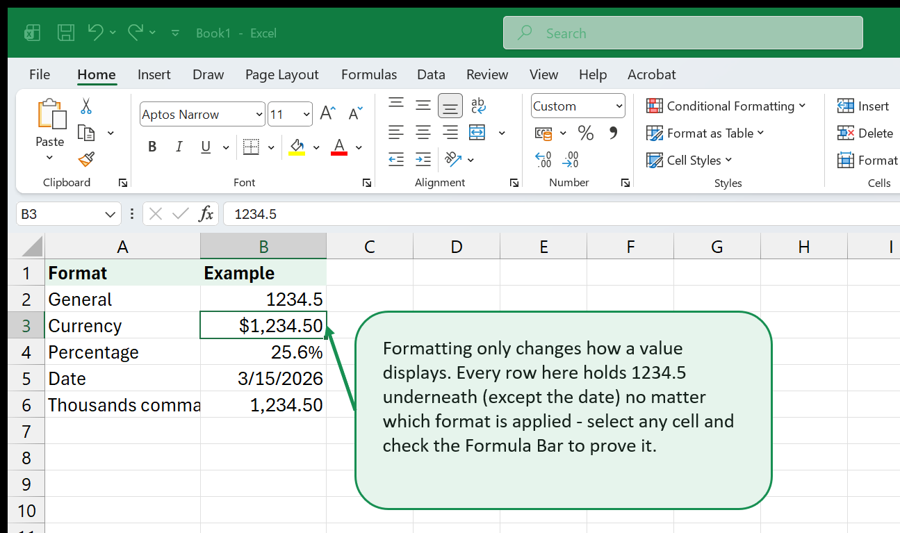
The Number group on the Home tab has quick buttons for the formats you’ll use constantly: Currency, Percentage, and Comma (thousands separator). The small dropdown next to them (defaults to “General”) opens the full list, including Date formats and a “More Number Formats” option for anything custom. A few notes that save real confusion later:

• Percentages are stored as decimals. Formatting a cell as a percentage displays 0.25 as 25%, but the stored value is still 0.25 - so a formula like =A1*B1 where B1 shows 25% is really multiplying by 0.25, which is exactly what you want, but it trips people up the first time they type 25 into a percentage-formatted cell expecting it to mean 25% (it becomes 2500% instead - type 0.25, or type 25% with the percent sign included, and Excel converts it correctly either way).
• Dates are stored as serial numbers counting days from a fixed start point (January 1, 1900 on Windows). This is why you can do math on dates - =B2-A2 between two date cells returns the number of days between them - and why a date can look like a five-digit number if the cell’s format ever gets reset to General by accident.
• Cell Styles (Home tab, to the right of Number) apply a whole bundle of formatting - font, fill color, borders - in one click, and keep a consistent look across a workbook without you manually matching colors cell by cell.

6. Rows, Columns, and Freeze Panes

Right-click a row number or column letter to Insert, Delete, or set an exact Row Height / Column Width. Double-click the thin border between two column letters (or two row numbers) to auto-fit that column or row to its contents - faster than dragging when you just want text to stop getting cut off.

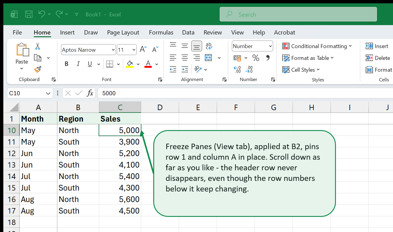
Freeze Panes (View tab) is the fix for the most common frustration in long lists: scrolling down loses the header row, so you can no longer tell what column D actually means. Select the cell just below and to the right of what you want frozen - B2 freezes row 1 and column A - then choose Freeze Panes. Everything above and to the left of that cell stays fixed on screen no matter how far you scroll.

To undo it, the same menu now shows “Unfreeze Panes.” Split (right next to Freeze Panes on the View tab) is a related but different tool - it divides the window into independently-scrollable sections rather than locking anything in place, which is occasionally useful for comparing two distant parts of the same sheet side by side.

7. Printing and Page Setup

Excel sheets are not naturally page-shaped, so what prints is not always what you expect until you’ve set it up once. Page Layout view (View tab, or the icon in the bottom-right corner) shows margins and page breaks directly on screen while you edit - it is the fastest way to see what will actually print, without opening Print Preview separately.

The Page Layout ribbon tab controls the details:

• Margins, Orientation, Size - the basics. Landscape is usually the right call for anything wider than about eight columns.
• Print Area (in the Page Setup group) - restricts printing to a specific selected range, so Excel doesn’t try to print every stray cell you’ve ever touched on that sheet.
• Print Titles - lets you repeat a specific header row (or column) on every printed page, which matters the moment a list runs past one page; without it, page two of a printed report has numbers with no labels.
• Scale to Fit (in the same group) - shrinks the printed output to fit a set number of pages wide/tall, which is usually a better fix for “my table is one column too wide for the page” than manually narrowing columns.

Ctrl+P opens Print, which includes a live preview - always check it before printing anything more than a page or two, since it catches most surprises (a stray extra page, a table cut awkwardly in half) before paper is wasted.

8. How Formulas Work: Operators and Order of Operations

Every formula starts with an equals sign (=) - that’s the signal to Excel that what follows is something to calculate, not text to display literally. Leave off the = and Excel just stores 2+3*4 as a text string.

The basic math operators: + add, - subtract, * multiply, / divide, ^ exponent (so =2^3 is 8). Comparison operators - =, <, >, <=, >=, <> (not equal) - return TRUE or FALSE and show up constantly inside functions like IF (Chapter 11).

Excel follows the same order of operations you learned in school: parentheses first, then exponents, then multiplication and division (left to right), then addition and subtraction (left to right) - often remembered as PEMDAS. This means =2+3*4 is 14, not 20, because the multiplication happens before the addition. Wrap the part you want done first in parentheses to force the order you actually mean:

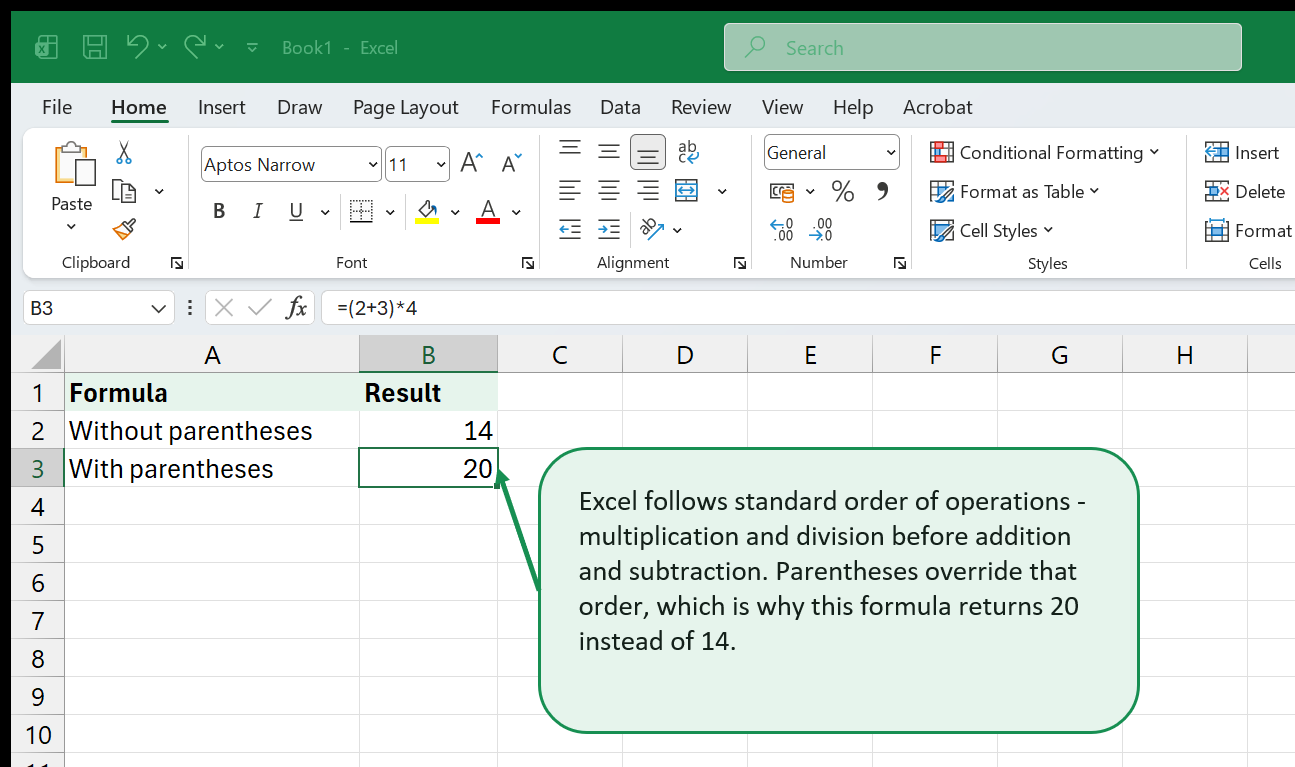
This one habit - adding parentheses even when you’re fairly sure you don’t strictly need them - prevents a large share of “why is this formula wrong” confusion, because it makes your intent explicit instead of relying on correctly remembering precedence rules under pressure.

9. Relative vs. Absolute References ($ signs explained)

This is the idea that unlocks everything else in this book, so read it twice if the first pass doesn’t fully land.

When you copy a formula to a new cell, Excel shifts its cell references to match - =A2*B2 copied down one row becomes =A3*B3 automatically. This is relative referencing, and it’s the default, and it’s usually exactly what you want: a total column where every row multiplies its own quantity by its own price.

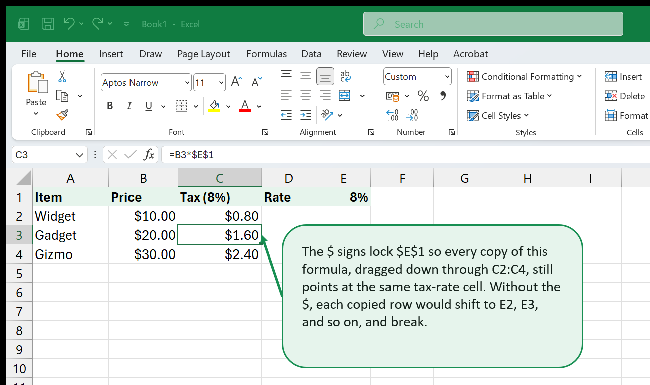
But sometimes a formula needs to keep pointing at the same cell no matter where it’s copied - a tax rate, a fixed fee, an exchange rate stored once at the top of the sheet. For that, add a dollar sign before the column letter, the row number, or both: $E$1 never shifts, in either direction, no matter where the formula is copied. This is an absolute reference.

You can also lock just one half - $E1 keeps the column fixed but lets the row shift, E$1 keeps the row fixed but lets the column shift - useful in two-directional tables, though $E$1 (locking both) covers the large majority of real cases. Press F4 while a cell reference is selected inside a formula to cycle through all four combinations without retyping the dollar signs by hand.

10. Five Functions Everyone Should Know: SUM, AVERAGE, COUNT, MAX, MIN

A function is a formula with a name: instead of writing out =B2+B3+B4+B5, you write =SUM(B2:B5) and let Excel do the addition. Every function follows the same shape - a name, then parentheses containing its arguments, separated by commas.

These five cover most everyday arithmetic:

• SUM(range) - adds every number in the range.
• AVERAGE(range) - the mean.
• COUNT(range) - counts how many cells in the range contain a number (not text, not blanks - see COUNTA if you need to count non-blank cells of any type).
• MAX(range) / MIN(range) - the largest or smallest value.

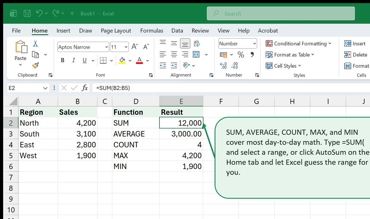
The fastest way to use any of them: select a cell below or beside a range of numbers, click AutoSum (the Greek-sigma Σ button on the Home tab, far right) and Excel guesses the adjacent range and inserts =SUM(...) automatically - click the small dropdown arrow next to AutoSum for AVERAGE, COUNT, MAX, and MIN as one-click options too. You can always edit the range afterward if Excel guessed slightly wrong.

11. Simple Logic: IF and IFS

IF tests a condition and returns one value if it’s true, another if it’s false: =IF(condition, value_if_true, value_if_false).

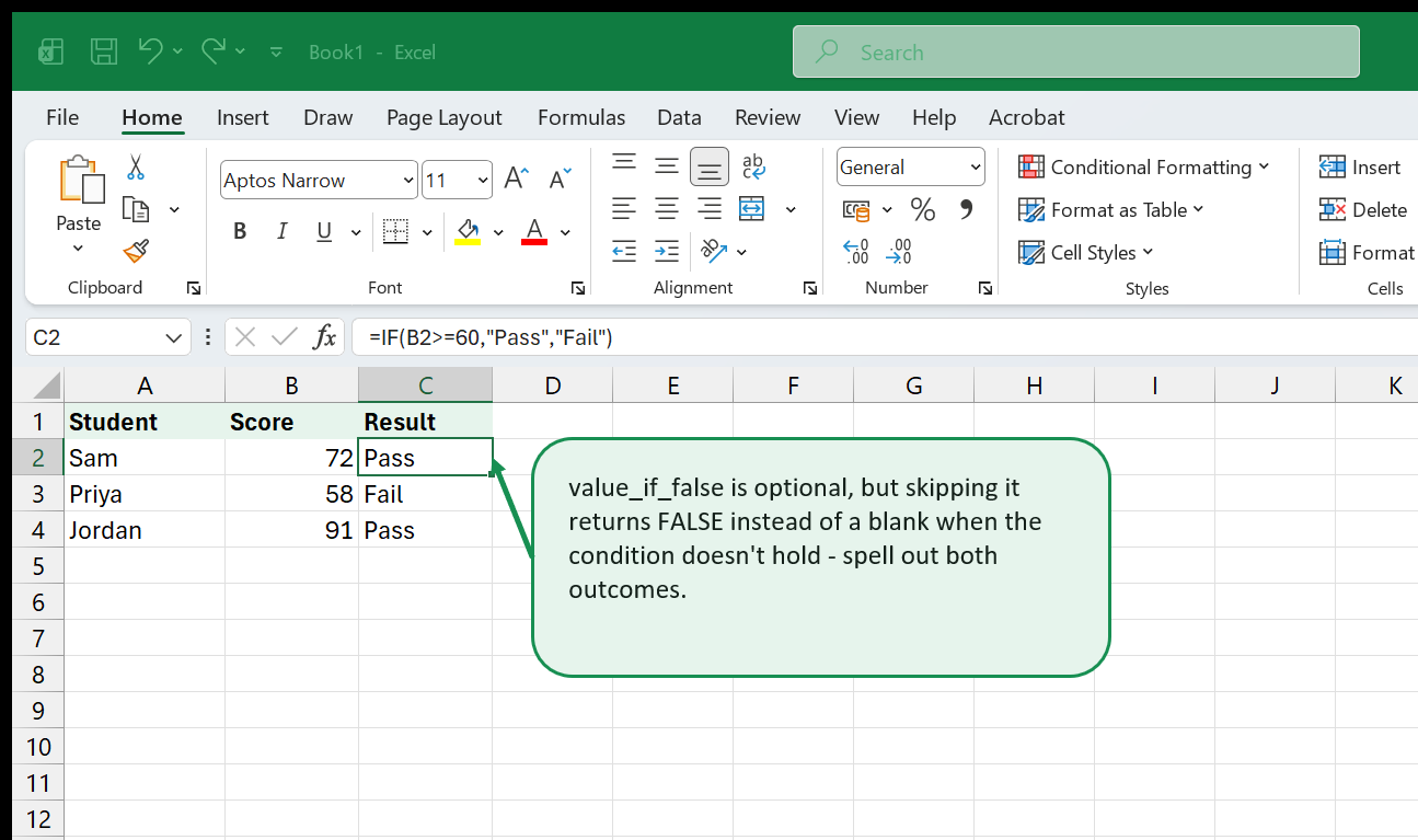
Always fill in value_if_false explicitly, even when it feels redundant. Leaving it out doesn’t leave the cell blank the way you might expect - it returns the word FALSE instead, which is rarely what you actually want to display.

IFS (available in Excel 2019 and Excel 365) extends the same idea across more than two outcomes, without nesting several IFs inside each other: =IFS(condition1, result1, condition2, result2, ..., TRUE, fallback). A grading formula that checks several score bands reads far more clearly as one IFS than as three or four nested IFs stacked inside one another.

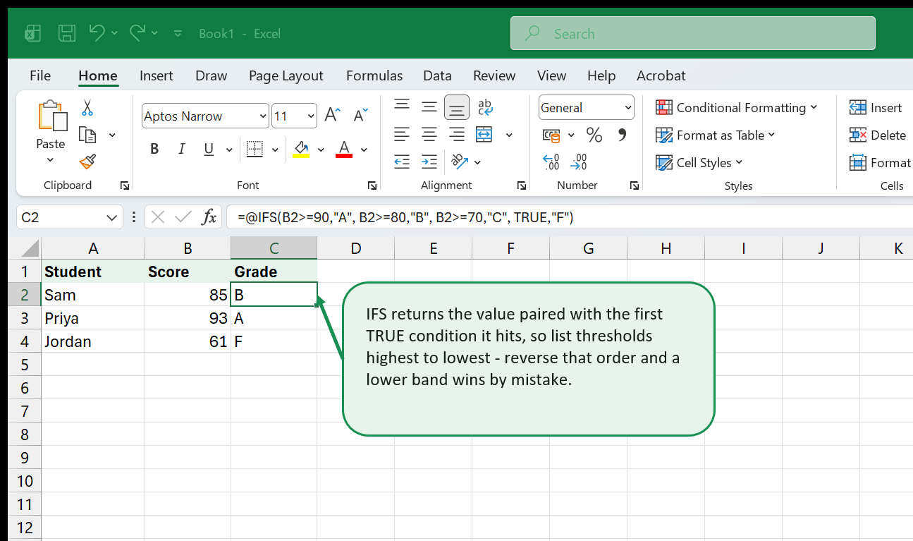
The one rule that trips people up: IFS returns the value paired with the first condition it finds true, and stops checking after that - so list conditions from the strictest (highest score) down to the loosest, always ending with a catch-all TRUE branch. Reverse that order, and a “B” band condition placed before the “A” band condition will claim scores that should have earned an “A.”

12. Your First Lookup: VLOOKUP and XLOOKUP

A lookup formula finds a value in one place and returns something related to it from another place - the single most useful category of formula for anyone working with lists of data (products and prices, employees and departments, order numbers and statuses).

VLOOKUP is the classic version: =VLOOKUP(lookup_value, table_array, col_index_num, [range_lookup]). It searches down the first column of table_array for lookup_value, then returns a value from the column you specify by position - col_index_num counts columns from the left edge of table_array itself, not from the worksheet.

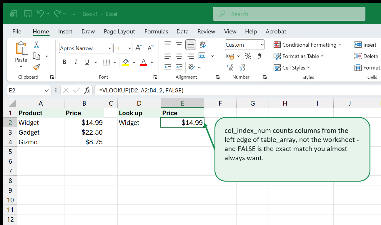
Set the fourth argument to FALSE (or 0) almost every time - it forces an exact match. Leaving it blank or setting TRUE tells Excel to accept the closest match if an exact one isn’t found, which is rarely what you want for looking up products, names, or IDs, and is the single most common source of a VLOOKUP silently returning the wrong row instead of a clear error.

XLOOKUP (Excel 365 and Excel 2021+) is the modern replacement: =XLOOKUP(lookup_value, lookup_array, return_array). It defaults to an exact match (no FALSE to remember), can search in either direction, and has a built-in if_not_found argument so you can skip wrapping it in a separate IFERROR. If your Excel version has it, prefer XLOOKUP for new work; VLOOKUP is still worth knowing since it appears throughout older workbooks you’ll inevitably inherit.

13. Sorting, Filtering, and Excel Tables

Sorting rearranges rows by a column’s values - select your data, then Data tab > Sort (or the A-Z / Z-A quick buttons for a single-column sort). Always sort with headers included and “My data has headers” checked, or Excel may try to sort your header row along with everything else.

Filtering hides rows that don’t match a condition, without deleting or reordering anything - Data tab > Filter adds a small dropdown arrow to each header cell, and unchecking values (or using the text/number filter options) hides the rest instantly. Filtered rows come back the moment you clear the filter.

The fastest way to get both, permanently, on a growing list: select your data and press Ctrl+T (or Insert > Table) to convert it into a proper Excel Table. A Table adds the sort/filter dropdown arrows to every header automatically, and - more importantly - any formula referencing the table auto-extends to new rows the moment you type them, without you having to drag a fill handle down manually every time the list grows.

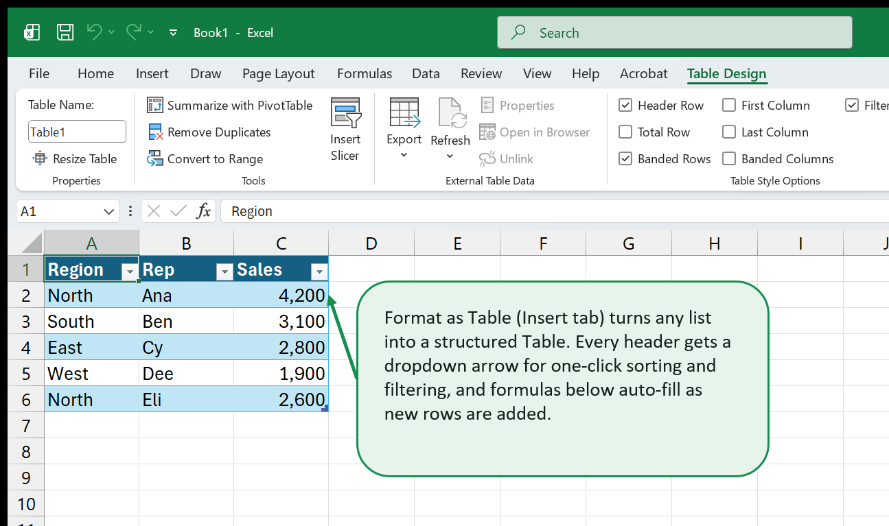
Tables also give each column a plain-English name usable in formulas (this is called a structured reference, e.g. =SUM(Table1[Sales]) instead of =SUM(C2:C50)) - worth knowing exists, even if you don’t reach for it on day one.

14. Removing Duplicates and Cleaning Messy Data

Real-world data is rarely clean: extra spaces from a copy-paste, the same customer entered twice with slightly different capitalization, numbers that imported as text. A few tools handle the most common problems:

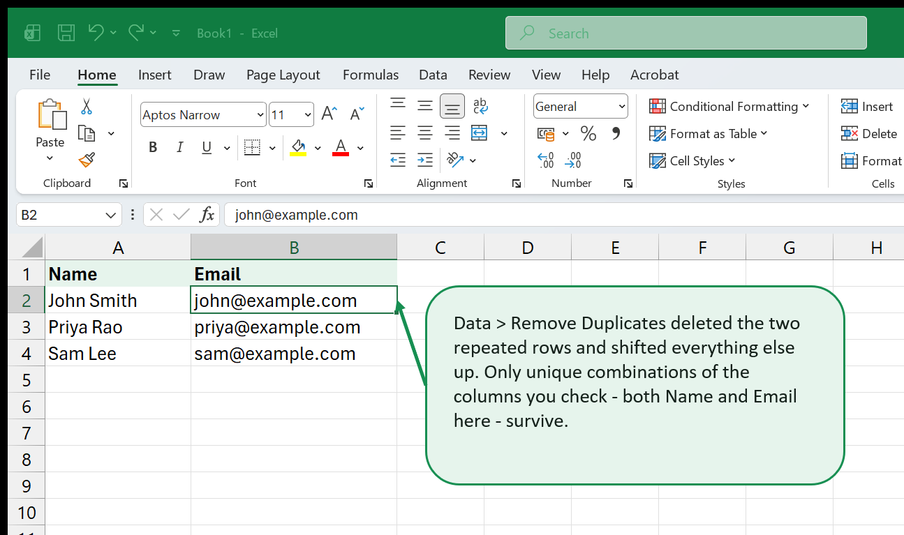
• Remove Duplicates (Data tab) deletes rows that repeat, based on whichever columns you check in its dialog - check every column that should match for a row to count as a true duplicate, since checking fewer columns treats near-duplicates as identical more aggressively than you may intend.

• TRIM(text) removes extra spaces from text - leading, trailing, and multiple spaces collapsed to one - the single highest-value cleanup formula for imported or pasted data, since invisible extra spaces are a common reason two values that look identical don’t match in a lookup or a duplicate check.
• PROPER(text), UPPER(text), LOWER(text) fix inconsistent capitalization.
• Text to Columns (Data tab) splits one column into several based on a delimiter (a comma, a space) - the fast fix for a “Full Name” column that should really be separate First and Last columns.
• Number stored as text shows up as a small green triangle in the corner of a cell, with a warning icon offering “Convert to Number” - a common, confusing cause of SUM silently ignoring a column of numbers that look fine but don’t add up.

None of these need to be memorized in depth on a first read - knowing they exist, and which problem each one solves, is enough to know where to look when messy data shows up.

15. Your First Chart and Conditional Formatting

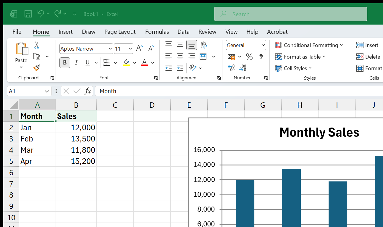
Charts turn a table of numbers into a picture. Select your data (include the header row) and press Alt+F1 for an instant default chart on the same sheet, or use Insert > Charts to pick a specific type deliberately. Excel usually guesses a sensible chart type from the shape of your data - a clustered column chart for a short category-by-value table like months and sales - and the chart updates live if the underlying numbers change later.

Conditional Formatting (Home tab) changes a cell’s appearance automatically based on its value, without you touching the Fill Color button by hand. The most useful presets:

• Color Scales - shades every cell on a gradient from low to high (or three-color, low/middle/high) - ideal for scanning a column of scores or results at a glance.
• Data Bars - draws a small in-cell bar proportional to the value, turning a column of numbers into a miniature bar chart without a separate chart object.
• Highlight Cells Rules and Top/Bottom Rules - flag values above or below a threshold, duplicates, or the top/bottom N values or percentage, in one dialog.

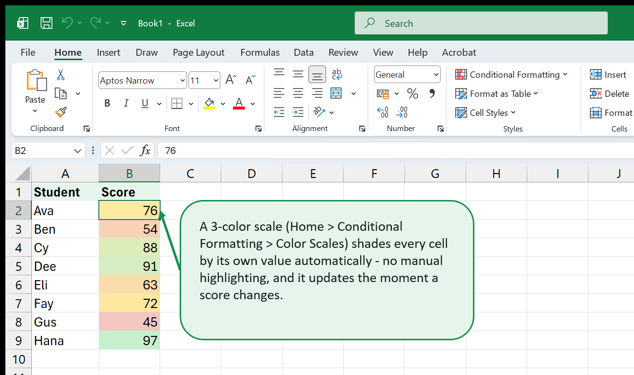
Every conditional format stays live - change a score, and its color updates immediately, with nothing to reapply by hand.

16. A Gentle Introduction to Pivot Tables

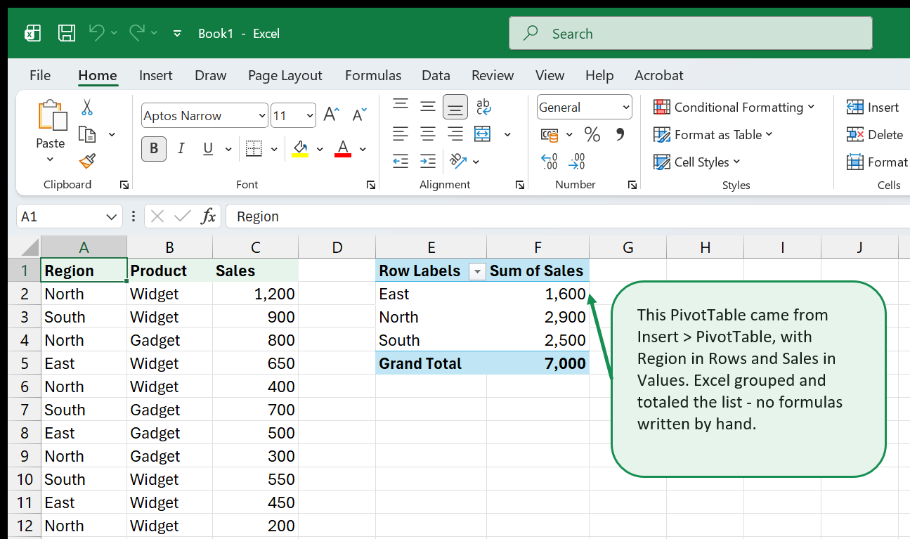
A PivotTable summarizes a long list - hundreds or thousands of rows - into a short, grouped, totaled table, without writing a single formula. This is the single biggest jump in capability for anyone who has outgrown SUMIF and manual totals.

To build one: click any cell inside your data, then Insert > PivotTable, and accept the default destination (a new sheet). A field list appears on the right with every column header from your source data. Drag the field you want to group by (say, “Region”) into the Rows area, and drag the field you want to total (say, “Sales”) into the Values area. Excel groups every matching row and totals it instantly.

A few things that make PivotTables feel less mysterious once you know them:

• Values defaults to Sum for numeric fields, but you can change it (click the field in the Values area > Value Field Settings) to Average, Count, Max, Min, and more.
• Dragging a second field into Rows nests it inside the first - Region, then Product within each Region, for example - without any extra setup.
• The source data doesn’t update the PivotTable automatically if you add new rows - right-click anywhere inside the PivotTable and choose Refresh after adding data, or the totals will look stale.
• A PivotTable never changes your original data. It’s a separate summary view built from it, which means there’s no risk in experimenting - dragging fields in and out to see what a different grouping looks like costs nothing, and can always be undone or rebuilt from scratch.

17. Common Errors Explained (#REF!, #VALUE!, #N/A, and more)

Every Excel error names the specific problem, which makes them far less intimidating once you know what each one is actually saying:

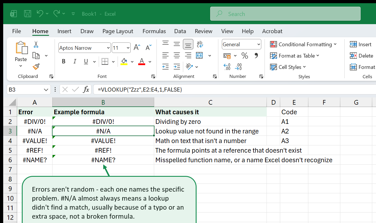
• #DIV/0! - the formula divided by zero, or by a cell that’s blank (which Excel treats as zero in arithmetic).
• #N/A - a lookup (VLOOKUP, XLOOKUP, MATCH) didn’t find a match. This is almost never a “broken” formula - it’s nearly always a genuine typo, an extra space, or mismatched capitalization/formatting between the lookup value and the data it’s searching. Check the actual values on both sides before assuming the formula itself is wrong.
• #VALUE! - the formula is trying to do math on something that isn’t a number - text where a number was expected, most commonly.
• #REF! - the formula points at a cell reference that no longer exists, usually because a row, column, or sheet it depended on was deleted.
• #NAME? - Excel doesn’t recognize something in the formula - most often a misspelled function name, or a reference to a named range that was never actually created.
• #SPILL! - a “spilling” formula (like FILTER or UNIQUE, which can return multiple results from one cell) found something already occupying the cells it needs to expand into. Clear that space and it resolves itself.

IFERROR(formula, value_if_error) catches any of these and substitutes a friendlier result - but use it deliberately, on a specific formula you’ve already confirmed works correctly for good data, not as a blanket habit for every formula. Wrapping a formula in IFERROR before it’s actually correct just hides genuine mistakes behind the same friendly fallback message, which makes them much harder to catch later.

18. Keyboard Shortcuts + Where to Go Next

A short list of the shortcuts worth actually memorizing - the ones that pay for themselves within the first week of regular use:

Shortcut	What it does
Ctrl+S	Save
Ctrl+Z / Ctrl+Y	Undo / Redo
Ctrl+C / Ctrl+X / Ctrl+V	Copy / Cut / Paste
Ctrl+Arrow	Jump to the edge of a data block
Ctrl+Home	Jump to cell A1
Ctrl+Page Up / Ctrl+Page Down	Switch sheet tabs
F2	Edit the selected cell in place
F4	Cycle relative/absolute references in a formula
Ctrl+T	Convert a range into a Table
Alt+F1	Insert a default chart from the selected data
Ctrl+1	Open Format Cells
Ctrl+Shift+L	Toggle Filter arrows on/off

Where to go next. This book is a linear on-ramp - the rest of excelback.com is the reference to come back to once a specific question comes up:

• Browse Excel topics for a structured path through any single skill area in more depth - Pivot Tables, Power Query, Charts, and more.
• Look up any function by name in the function reference - every function mentioned in this book has its own page there, with more examples.
• If you’d rather follow a longer, structured sequence of lessons instead of a single book, browse the course paths.
• Free templates and practice datasets are ready to download and use immediately - no sign-up, direct .xlsx files. A few that pick up exactly where a chapter here left off: the VLOOKUP / XLOOKUP practice dataset (Chapter 12), the messy data cleanup practice file (Chapter 14), the conditional formatting practice file (Chapter 15), and the PivotTable practice dataset (Chapter 16).

You now have the working vocabulary for almost everything else written about Excel. The fastest way to get comfortable from here is the most boring-sounding advice in this entire book: open a real workbook of your own and use it.