Data Cleaning in Excel

This guide is for anyone who has ever opened a CSV export and immediately felt their stomach drop. Maybe the dates are formatted wrong, product names are littered with extra spaces, customer records are duplicated, and three columns that should be one are crammed into a single field. That is the reality of working with real-world data — spreadsheets imported from point-of-sale systems, e-commerce platforms, or accounting software rarely arrive in a clean, analysis-ready state. Before you can build a pivot table, write a VLOOKUP, or draw a chart that actually means something, you have to fix the raw material.

This ebook walks you through a complete data cleaning workflow using a messy POS export as the running example. You will learn to identify every major category of dirty data, then apply the right Excel tools to fix each one — from the Data tab’s built-in commands to text functions you will reach for every single week. The techniques here apply equally to Excel 365, Excel 2019, and Excel 2021.

Work through the sections in order the first time. Once you know the workflow, the Quick Reference table at the end becomes your go-to cheat sheet for any future cleaning job.

---

Why Data Cleaning Comes Before Everything Else

Every analysis is only as reliable as its inputs. A duplicated sales row inflates your revenue figures. A stray space turns "Q1 Sales" into something that will never match a lookup value. A date stored as text means your timeline charts plot nothing at all.

The fundamental rule: never analyze data you have not cleaned. Resist the temptation to jump straight to calculations. Spend twenty minutes on the cleaning steps in this guide and you will avoid hours of debugging mysterious wrong answers later.

---

Spotting Dirty Data

Before touching a single formula, spend five minutes auditing your dataset. Cleaning problems you cannot see are problems you cannot fix.

Open your import file and work through this checklist:

Visual scan

• Scroll through every column. Do values look consistent in format, capitalization, and length?
• Check the first and last rows — imports often bury header rows or summary totals at the bottom.

Column-by-column checks

• Numeric columns: select the column and glance at the status bar (bottom right). If Sum shows 0 for a column that should total thousands, the values are stored as text.
• Date columns: are all values right-aligned (real dates) or left-aligned (text strings)?
• ID or code columns: use a quick sort to surface duplicates visually.

Row count check Use =COUNTA(A:A)-1 to count non-blank rows excluding the header. Compare this to the record count your source system reported on export. A mismatch signals missing or doubled rows.

Blank cell audit Select the entire data range, press Ctrl + G, click Special, then choose Blanks. Excel selects every empty cell. If you see blanks in columns that should be fully populated — order IDs, dates, product codes — you have gaps to investigate before proceeding.

---

Removing Duplicates

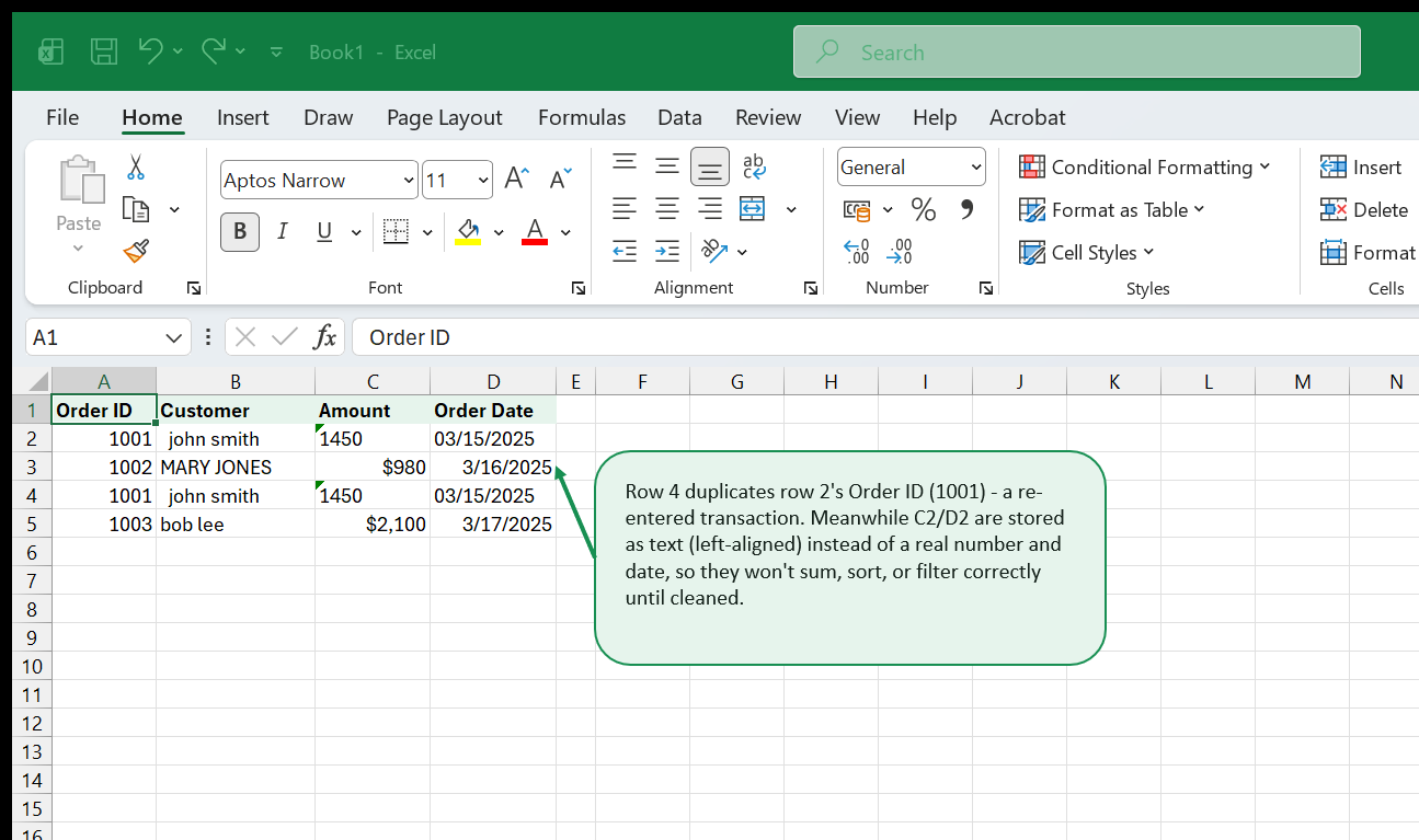
Duplicate rows are among the most common problems in POS exports, especially when a system allows a transaction to be voided and re-entered, or when data is exported across overlapping date ranges.

The built-in command

1. Click anywhere inside your data range.
2. Go to Data tab > Remove Duplicates.
3. In the dialog, check the columns that together define a unique record. For a sales export that is usually Order ID — not every column, because two orders can legitimately have the same amount or date.
4. Click OK. Excel reports how many duplicates were removed and how many unique rows remain.

Before you click OK, always copy your data to a backup sheet. Remove Duplicates is permanent — there is no undo that survives a file close.

Flagging before removing

If you want to review duplicates before deleting them, use COUNTIF to flag them first:

Add this formula in a helper column. Any row returning a value greater than 1 shares its Order ID with at least one other row. Filter on values greater than 1, review the flagged rows, then delete the ones you are confident are true duplicates.

---

Trimming Extra Spaces: TRIM and CLEAN

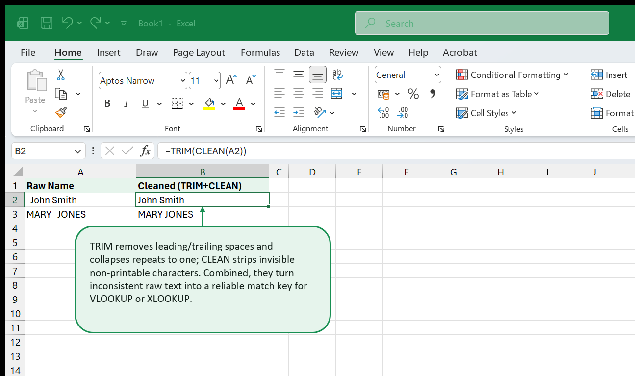
Extra spaces are invisible to the eye but catastrophic for formulas. "Q1 Sales " and "Q1 Sales" are different strings — a VLOOKUP or MATCH will find no match between them.

TRIM removes all leading spaces, trailing spaces, and reduces any runs of internal spaces down to a single space.

CLEAN removes non-printable characters — the invisible ASCII codes (characters 1–31) that sneak in when data is exported from legacy systems or copied from web pages.

The two functions combine perfectly:

Workflow: add a helper column with =TRIM(CLEAN(A2)), fill it down, then copy the entire helper column, paste as Values Only (Ctrl + Shift + V, then V) over the original column, and delete the helper column. This replaces the raw text with the clean version.

---

Fixing Capitalization: PROPER, UPPER, LOWER

Customer name fields exported from POS systems arrive in every capitalization imaginable — all-caps, all-lowercase, random mixed case. Excel’s three text-case functions standardize them instantly.

Function	What it does	Example input	Example output
PROPER	Capitalizes first letter of each word	"JOHN SMITH"	"John Smith"
UPPER	Converts all letters to uppercase	"widget"	"WIDGET"
LOWER	Converts all letters to lowercase	"WIDGET"	"widget"

Watch out for PROPER’s edge cases. It capitalizes the letter after any non-letter character, so "O'brien" becomes "O'Brien" (correct) but "Po box 123" becomes "Po Box 123" — the “b” in “box” is capitalized. Review PROPER output for product codes, abbreviations, or names with apostrophes before making it permanent.

Apply the same copy-paste-values workflow used for TRIM: helper column, fill down, paste as values, delete helper.

---

Splitting Columns: Text to Columns and Flash Fill

POS exports frequently pack multiple pieces of information into one cell — a full name in a single column, a city and state joined by a comma, a product code that embeds category and SKU. Splitting these out makes every downstream analysis far easier.

Text to Columns

Use Text to Columns when your data has a consistent delimiter (comma, tab, pipe, space) or a fixed width.

1. Select the column you want to split.
2. Go to Data tab > Text to Columns.
3. Choose Delimited (for comma-separated or similar) or Fixed Width.
4. Select the delimiter character — for a “City, State” column choose Comma.
5. Preview the result in the wizard, then click Finish.

Excel splits the values into adjacent columns, overwriting whatever is there. Make sure you have empty columns to the right before running the wizard.

Flash Fill

Flash Fill is faster for irregular patterns where a delimiter varies or doesn’t exist. In the column next to your data, type the result you want for the first row. Press Ctrl + E — Excel infers the pattern from your example and fills the rest of the column.

For a “FirstName LastName” column where you want only the first name, type the first name in the adjacent cell, then press Ctrl + E. Flash Fill reads your intent and extracts first names from every row.

Always review Flash Fill results — it occasionally misreads the pattern when data is inconsistent.

---

Combining Columns: TEXTJOIN and &

Sometimes the problem runs in the other direction: address fields split across five columns need to be assembled into one, or a product code needs a prefix appended.

The & operator concatenates values directly:

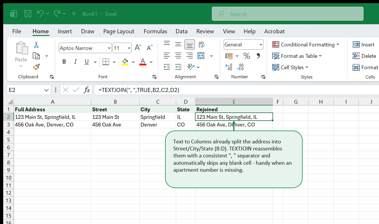
TEXTJOIN is more powerful for combining multiple cells with a separator, and it can skip blank cells automatically:

The first argument is the delimiter. The second argument (TRUE) tells TEXTJOIN to ignore empty cells — so if D2 (apartment number) is blank, you get "123 Main St, Springfield, IL" rather than "123 Main St, , Springfield, IL".

TEXTJOIN is available in Excel 2019, 2021, and 365. For older versions, use =A2&", "&B2&", "&C2 and handle blanks with IF statements.

---

Converting Text-as-Numbers to Real Numbers

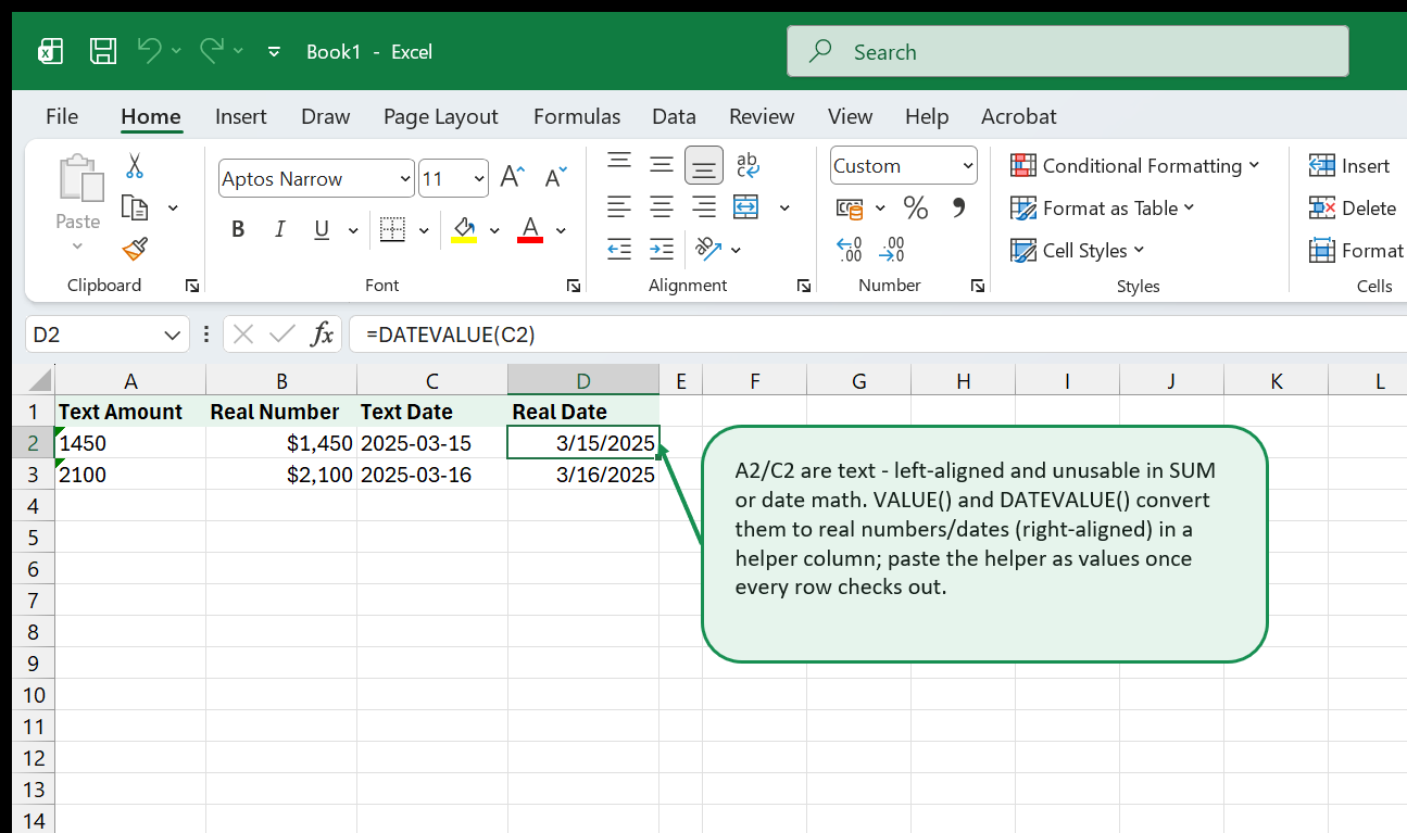
When Excel imports a CSV, it sometimes reads numeric columns as text. The telltale signs: values are left-aligned instead of right-aligned, the SUM of the column returns 0, or a small green triangle appears in the top-left corner of the cells.

Method 1: Error button

If the green triangles are present, click one of the flagged cells. A yellow warning icon appears to the left. Click it and choose Convert to Number. Then select all flagged cells and repeat.

Method 2: Paste Special multiply

Type the number 1 in any blank cell. Copy it. Select the text-number column. Go to Home tab > Paste > Paste Special (or Alt + E + S). Choose Multiply. Excel multiplies every selected cell by 1 — which forces them to evaluate as numbers without changing their values.

Method 3: VALUE function

Use VALUE in a helper column, fill down, then paste as values over the original. This works well when you want a clean audit trail before overwriting.

---

Fixing Broken Dates

Broken dates are among the trickiest cleaning problems because Excel handles dates as serial numbers internally. A date stored as text looks identical to a real date on screen but behaves completely differently in formulas and pivot tables.

Diagnosing the problem: select a suspect date cell. If the formula bar shows 03/15/2025 but the cell is left-aligned, or if =YEAR(A2) returns an error, the date is stored as text.

DATEVALUE converts a text date string to a real Excel date serial number:

The result looks like a large number — that is the Excel serial date. Format the cell as a Date (Ctrl + 1, then Number > Date) to display it correctly.

Inconsistent date formats are a separate headache. If your import contains a mix of MM/DD/YYYY and DD/MM/YYYY formats (common when data comes from international sources), you cannot fix them with a single formula. Sort the date column and visually identify which rows use which format. Use a helper column with an IF statement to detect and correct the ambiguous cases.

Text to Columns trick: selecting the date column and running Data > Text to Columns, clicking through the wizard without changing anything, and clicking Finish often forces Excel to re-parse text dates as real dates — especially for YYYY-MM-DD ISO format strings.

---

Using Find & Replace for Bulk Fixes

Find & Replace (Ctrl + H) is underrated as a cleaning tool. It works across the entire workbook or within a selection, and it handles several common problems in seconds.

Removing unwanted characters: to strip all dollar signs from a price column, open Find & Replace, type $ in the Find field, leave the Replace field blank, and click Replace All.

Standardizing inconsistent values: if your product category column contains both "Electronics" and "electronics" and "ELECTRONICS", you could use PROPER — but if there are only a handful of variants, Find & Replace is faster. Search for each variant and replace with the canonical form.

Replacing line breaks: imported data sometimes contains line breaks inside cells. In the Find field, press Ctrl + J to insert a line-break character (nothing will appear, but it is there). Leave Replace blank and click Replace All to strip them.

Using wildcards: check the Use wildcards checkbox to use * (any sequence of characters) and ? (any single character). To find any value starting with "SKU-" followed by anything, search for SKU-*.

---

Common Pitfalls

Knowing what can go wrong saves you from discovering it after you have already built a dashboard on dirty data.

Fixing data in place vs. in a helper column
Always build your cleaning formulas in a helper column first. Paste as values only when you have verified the output looks right for every row in your dataset, not just the first few.

Forgetting to fill down completely
When you write a formula in row 2 and fill down, it is easy to miss rows at the bottom if your dataset is large. After filling, press Ctrl + End to jump to the last cell in the used range and confirm your helper column extends all the way down.

Overwriting the original without a backup
Before any paste-as-values operation, duplicate the sheet (right-click the tab > Move or Copy > check Create a copy). Naming it "Raw Import" and keeping it hidden costs nothing and has saved countless analysts from disasters.

TRIM does not remove non-breaking spaces
Non-breaking spaces (ASCII 160, common in web-page pastes) are not removed by TRIM. If TRIM is not working, try =TRIM(SUBSTITUTE(A2,CHAR(160)," ")) to replace them first.

Date locale mismatches
DATEVALUE interprets date strings according to your system locale. On a US locale system, "03/15/2025" is March 15. On a UK locale system, it is interpreted as the 3rd of the 15th month — which is an error. If you share files across regional settings, use DATE(YEAR(...),MONTH(...),DAY(...)) to construct dates explicitly.

---

Quick Reference

Function	Syntax	What it does	Typical use
TRIM	=TRIM(text)	Removes leading, trailing, and extra internal spaces	Clean any text field on import
CLEAN	=CLEAN(text)	Removes non-printable characters	Legacy system exports
PROPER	=PROPER(text)	Title Case	Customer name fields
UPPER	=UPPER(text)	ALL CAPS	Product codes, category columns
LOWER	=LOWER(text)	all lowercase	Email addresses
VALUE	=VALUE(text)	Converts text-number to real number	Price, quantity columns stored as text
DATEVALUE	=DATEVALUE(text)	Converts text date to Excel date serial	Date fields stored as text
TEXTJOIN	=TEXTJOIN(delim, skip_blanks, text1, ...)	Joins multiple cells with a separator	Reassembling split address fields
SUBSTITUTE	=SUBSTITUTE(text, old, new)	Replaces every instance of a string	Removing characters TRIM cannot catch
COUNTA	=COUNTA(range)	Counts non-blank cells	Row count audit
COUNTIF	=COUNTIF(range, criteria)	Counts cells matching a value	Duplicate detection

Keyboard shortcuts for cleaning

Action	Shortcut
Open Find & Replace	Ctrl + H
Open Go To Special	Ctrl + G, then Alt + S
Fill selection down	Ctrl + D
Paste as Values	Ctrl + Shift + V, then V
Open Format Cells	Ctrl + 1
Jump to last used cell	Ctrl + End

---

Where to Go Next

Once your data is clean, the next step is building the analyses and automations that make it useful:

• Excel Formulas Cheat Sheet — a complete reference for lookup, text, date, math, and logical functions, with examples ready to drop into your workbook.
• Pivot Tables from Zero — once your data is clean, pivot tables are the fastest way to summarize it. This guide covers every option from grouping to calculated fields.
• XLOOKUP & VLOOKUP Field Guide — clean data plus a reliable lookup function is the foundation of almost every Excel reporting workflow. XLOOKUP replaces VLOOKUP with a cleaner syntax and fewer gotchas.

Want to practice on real messy data instead of the small examples above? Download the messy data cleanup practice dataset - extra whitespace, mixed case, duplicate rows, and numbers stored as text, deliberately, so you can run this entire workflow end to end. The text functions practice dataset does the same for TRIM, PROPER, and TEXTJOIN specifically on contact records.