XLOOKUP & VLOOKUP Field Guide

This is a reference, not a tutorial - open it when you need a specific lookup pattern, copy the formula, adjust the ranges, done. If you’ve never written a lookup formula before, read Chapter 12 of Excel for Beginners first; everything here assumes you already know what VLOOKUP and XLOOKUP are for.

Every formula below has been checked by hand for correct syntax and correct behavior, not just copied from memory. Ranges like A2:A5 are examples - swap in your own.

Which One to Use: XLOOKUP vs. VLOOKUP vs. INDEX/MATCH

Situation	Reach for	Why
Exact match, Excel 365 or 2021+	XLOOKUP	Defaults to exact match, searches either direction, has built-in not-found handling
Exact match, Excel 2019 or older	VLOOKUP or INDEX/MATCH	XLOOKUP isn’t available in those versions
Need to return a value to the left of the lookup column	INDEX/MATCH or XLOOKUP	VLOOKUP can only search its first column and return from columns to the right
Two-way lookup (row + column)	INDEX/MATCH (double MATCH) or nested XLOOKUP	Both work; INDEX/MATCH runs in every Excel version
Multiple criteria (two or more conditions)	XLOOKUP’s array trick, or INDEX/MATCH with an array formula	VLOOKUP has no native multi-criteria support
Approximate match against sorted brackets (tax, commission, grading)	VLOOKUP(...,TRUE) or XLOOKUP with match_mode	See the sorting caveat below - it differs between the two
Columns get inserted or deleted in the source table often	INDEX/MATCH or XLOOKUP	VLOOKUP’s col_index_num is a hardcoded position that silently breaks when columns shift; the other two reference columns by range
A huge lookup table and speed matters	XLOOKUP or MATCH with binary search_mode	Can outperform VLOOKUP on large sorted ranges

The short version: if your Excel has XLOOKUP (365 or 2021+), use it for new work by default. Keep VLOOKUP and INDEX/MATCH in your toolkit anyway - you will inherit workbooks that use both for as long as you work in Excel.

Exact-Match Lookups

The most common lookup of all: find a value, return the matching row’s data.

FALSE (or 0) as the fourth argument forces an exact match. col_index_num (the 2 above) counts columns from the left edge of table_array itself, not from the worksheet - a table_array of C2:F10 counts its own column C as 1, D as 2, and so on.

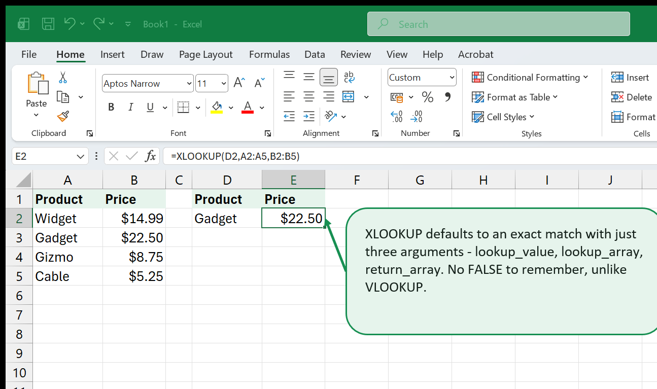
XLOOKUP defaults to exact match with only three required arguments - lookup_value, lookup_array, return_array. There’s no TRUE/FALSE argument to remember, and lookup_array and return_array are two separate ranges rather than one table_array, so they don’t need to sit next to each other or in any particular left-to-right order.

INDEX/MATCH does the same job in two steps: MATCH finds the position of D2 within A2:A5 (the 0 forces exact match, same idea as VLOOKUP’s FALSE), and INDEX returns the value at that position from B2:B5. It looks more roundabout than VLOOKUP, but the two ranges are fully independent, which is exactly what makes the next several patterns possible.

Approximate-Match / Range Lookups

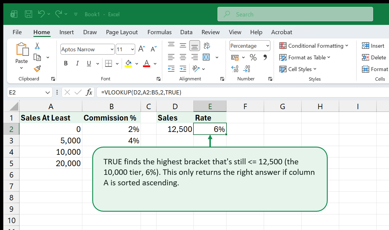
Use this whenever you’re matching a number against sorted brackets - tax tables, commission tiers, grading scales - rather than looking for an exact value. The formula should return the bracket whose threshold is the largest one ≤ the lookup value.

TRUE (or simply omitting the fourth argument) tells VLOOKUP to accept the closest match ≤ the lookup value when there’s no exact one. This requires table_array’s first column to be sorted ascending. Unsorted data doesn’t raise an error here - it just returns a confidently wrong bracket, which is the single most dangerous mistake in this entire guide.

match_mode -1 means “exact match, or the next smaller item” - the same behavior as VLOOKUP(...,TRUE). The genuine improvement: XLOOKUP’s default search (search_mode 1) scans in order and does not require the data to be pre-sorted for match_mode -1/1 to return the right answer. Only the binary-search modes (search_mode 2 or -2, an explicit opt-in for speed on very large sorted ranges) require sorted data - the default doesn’t.

Two-Way Lookups (Row + Column)

A two-way lookup returns the value at the intersection of a row match and a column match - a small grid of products by month, say, where you want one specific cell without scrolling to find it.

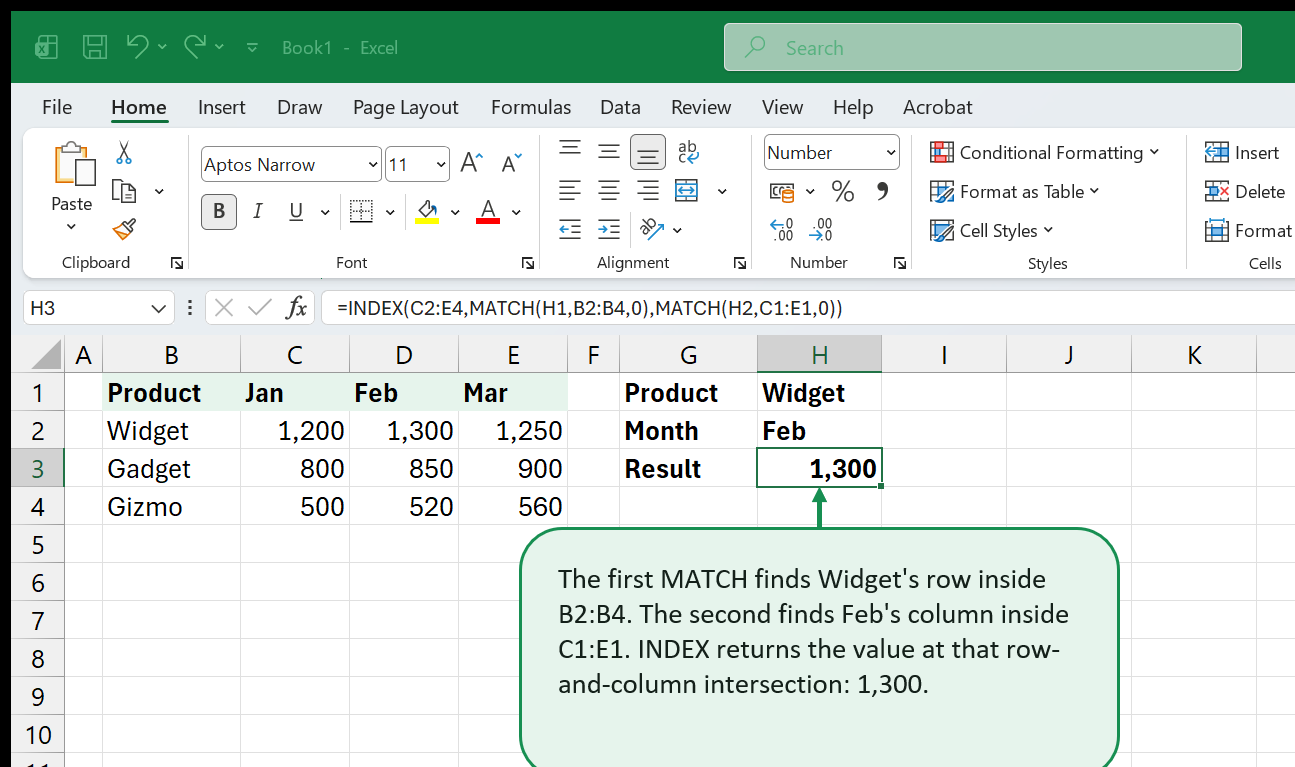
INDEX’s optional third argument - column_num - is what makes this work. The first MATCH finds which row H1 (a product) is at within B2:B4; the second finds which column H2 (a month) is at within C1:E1. INDEX then returns the cell at that row-and-column position inside C2:E4. This pattern runs in every Excel version, including ones without XLOOKUP.

A single XLOOKUP only searches one dimension, so a two-way lookup nests two of them. The inner XLOOKUP finds which column H2 matches within C1:E1, then returns that entire matching column from C2:E4 as an array. The outer XLOOKUP then searches B2:B4 for H1 and returns the matching row from that inner array. Read it inside-out: the column lookup happens first, the row lookup happens second, against whatever the column lookup handed back.

Multi-Criteria Lookups

Two reliable ways to match on more than one condition at once - neither needs an array-entered {} formula in a current Excel version.

Helper column (works with plain VLOOKUP, the simplest to explain to a coworker): add a column that concatenates every criterion into one key, immediately to the left of what you want to return, then look up against the combined key.

The | is just a separator unlikely to appear in real data - anything works, as long as it can’t accidentally make two different criteria pairs produce the same combined key (e.g. "AB"&"C" and "A"&"BC" would collide without a separator).

Array trick, no helper column (works with XLOOKUP and INDEX/MATCH, not with VLOOKUP): multiply two boolean comparisons together. Each comparison produces an array of TRUE/FALSE, treated as 1/0; the product is 1 only where every condition is true for that row.

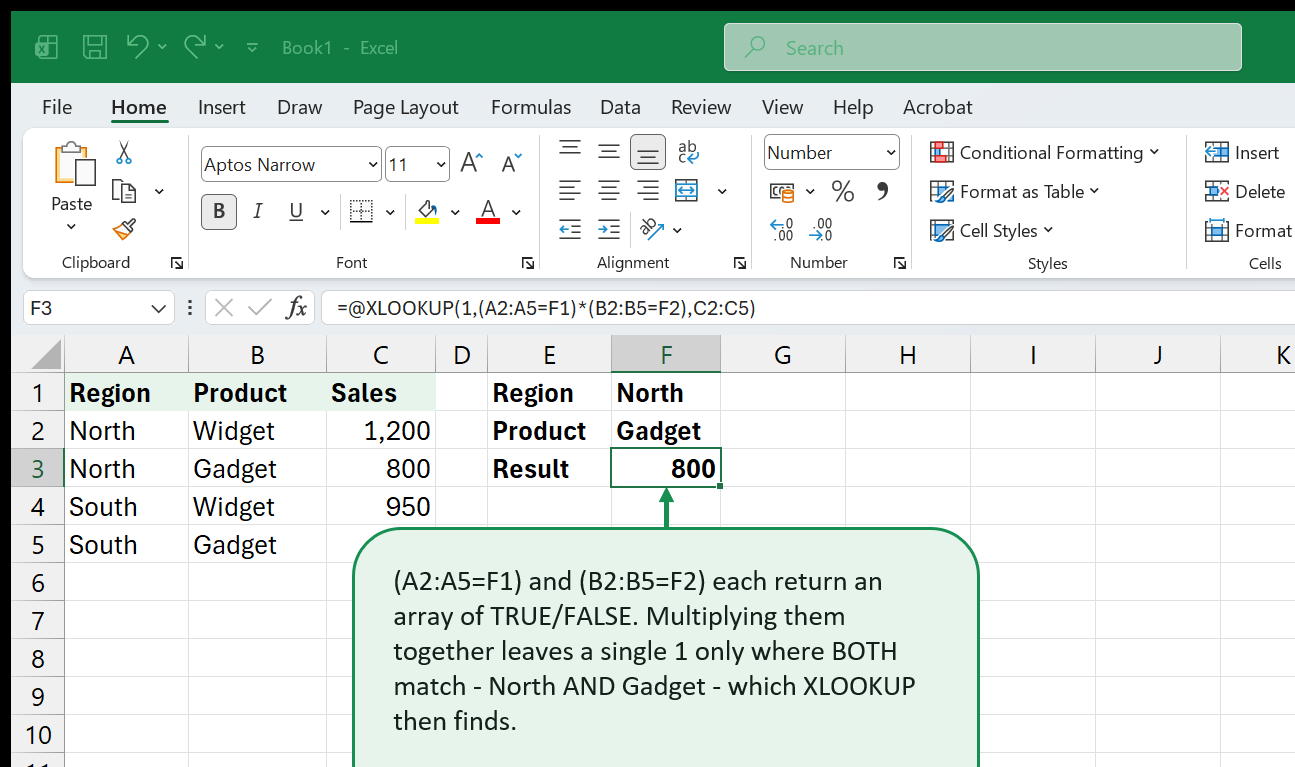
(A2:A5=F1) returns an array like {1,1,0,0} (region matches), (B2:B5=F2) returns {0,1,0,1} (product matches), and multiplying them gives {0,1,0,0}

• exactly one 1, at the row that satisfies both. XLOOKUP then looks for that 1 and returns the matching row’s value. The INDEX/MATCH version of the same idea:

Add a third criterion by multiplying in a third comparison the same way - (A2:A5=F1)*(B2:B5=F2)*(D2:D5=F3).

Lookups in Either Direction

VLOOKUP always searches the first column of table_array and returns from a column to its right - it cannot return a value from a column to the left of the one it searched. This trips people up constantly when a source table happens to have the lookup key in, say, column C and the value they actually want in column A.

INDEX/MATCH and XLOOKUP don’t have this limitation at all, because lookup_array and return_array are two entirely independent ranges - they can point in either direction, or even at different sheets.

Both formulas search column C for an ID and return the corresponding value from column A, to its left - something no version of VLOOKUP can do without physically rearranging the source columns first.

Wildcard Matches

* matches any number of characters, ? matches exactly one - both work in exact-match lookups, useful for “starts with,” “contains,” or “any single character differs” style matches.

VLOOKUP supports wildcards automatically in its exact-match (FALSE) mode

• nothing extra to turn on.

XLOOKUP needs match_mode 2 set explicitly - its default exact match (match_mode 0) treats * and ? as literal characters, not wildcards.

If the data you’re searching genuinely contains a literal * or ? (not as a wildcard), escape it with a tilde: ~* or ~? finds the actual character.

Handling “Not Found” Gracefully

A lookup that finds nothing returns #N/A by default. Three ways to handle that cleanly, in order of how deliberately they narrow what they catch:

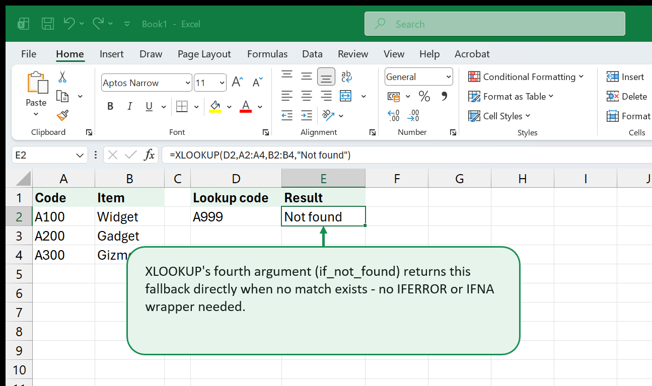
XLOOKUP’s fourth argument, if_not_found, handles this natively - the cleanest option when it’s available, since there’s no separate wrapper formula to add or maintain.

IFERROR catches any error the inner formula produces, not just “no match.” That’s exactly the risk: wrapping a formula in IFERROR before you’ve confirmed it works correctly on good data hides genuine mistakes - a typo’d range, say - behind the same friendly fallback text a real not-found result would show.

IFNA only catches #N/A - a genuinely missing lookup value - and lets any other error (a #REF! from a deleted column, for instance) through unmasked, where it’s still visible enough to notice and fix. Prefer IFNA over a blanket IFERROR on a lookup formula for exactly that reason.

Common Pitfalls & Quick Fixes

• VLOOKUP’s fourth argument defaults to TRUE if omitted. Type FALSE explicitly every time you want an exact match - which is almost always.
• col_index_num breaks silently when a column is inserted into table_array - the number doesn’t update, so the formula keeps returning whatever now sits at that position instead of what you originally meant. INDEX/MATCH and XLOOKUP don’t have this problem; they reference columns by range, not by counted position.
• Text that looks like a number doesn’t match a real number. A lookup_value of "102" (text) will not match a cell holding the number 102. This is the same “number stored as text” issue covered in Excel for Beginners, and it’s a common, confusing cause of a lookup that looks correct but returns #N/A anyway.
• A trailing space breaks an otherwise-perfect match. Copy-pasted or imported text often carries an invisible space at the end. Wrap the lookup value (or the source column) in TRIM() if a match keeps failing for no visible reason.
• VLOOKUP(...,TRUE) on unsorted data returns a wrong answer, not an error - the single most dangerous mistake on this page, because nothing ever tells you it happened. Sort the bracket table ascending, always.
• Whole-column references (A:A) are convenient and fine for normal workbook sizes; on very large sheets, narrowing to the actual data range (A2:A50000) keeps recalculation snappier.

Quick Reference: Every Pattern at a Glance

Pattern	Formula
Exact match (XLOOKUP)	=XLOOKUP(lookup_value, lookup_array, return_array)
Exact match (VLOOKUP)	=VLOOKUP(lookup_value, table_array, col_index_num, FALSE)
Exact match (INDEX/MATCH)	=INDEX(return_range, MATCH(lookup_value, lookup_range, 0))
Approximate match (VLOOKUP, needs sorted data)	=VLOOKUP(lookup_value, table_array, col_index_num, TRUE)
Approximate match (XLOOKUP, sort not required)	=XLOOKUP(lookup_value, lookup_array, return_array, , -1)
Two-way lookup (INDEX/MATCH)	=INDEX(grid, MATCH(row_val, row_headers, 0), MATCH(col_val, col_headers, 0))
Two-way lookup (nested XLOOKUP)	=XLOOKUP(row_val, row_headers, XLOOKUP(col_val, col_headers, grid))
Multi-criteria (helper column)	=VLOOKUP(key1&key2, helper_range, n, FALSE)
Multi-criteria (array, no helper)	=XLOOKUP(1, (range1=crit1)*(range2=crit2), return_range)
Lookup to the left	=INDEX(return_range, MATCH(lookup_value, lookup_range, 0))
Wildcard (VLOOKUP)	=VLOOKUP("text*", table_array, col_index_num, FALSE)
Wildcard (XLOOKUP)	=XLOOKUP("text*", lookup_array, return_array, , 2)
Not found (XLOOKUP built-in)	=XLOOKUP(lookup_value, lookup_array, return_array, "fallback")
Not found (IFNA, N/A only)	=IFNA(lookup_formula, "fallback")
Not found (IFERROR, any error)	=IFERROR(lookup_formula, "fallback")

Where to Go Next

Every function in this guide has its own full reference page, with more examples than fit here: XLOOKUP, VLOOKUP, INDEX, MATCH, XMATCH, HLOOKUP, and IFERROR.

• Download the VLOOKUP / XLOOKUP practice dataset
  • a 20-row product table plus a questions sheet, built to practice exactly the patterns in this guide with both functions.
• The Formula Builder and Formula Explainer tools help construct or decode a lookup formula without leaving the browser.
• The Formulas & Functions course path and the Formulas & Functions topic go deeper on everything else in this function category.
• New to formulas entirely? Start with Excel for Beginners, the free starting point this guide assumes you’ve already read.
• Need SUM, COUNT, or text-cleanup syntax instead of lookups? The Excel Formulas Cheat Sheet covers every function category on this site in the same condensed format.