Date & Time Functions Guide

Dates and times trip up more Excel users than almost any other topic. You paste a date from a website and Excel shows a number. You subtract two dates and wonder why the result is a fraction. You need to count only working days between two milestones but DAYS() counts weekends too. The root of nearly every date frustration is the same: Excel stores dates as plain numbers, and once you understand that, the entire function family clicks into place.

This guide covers every major date and time function in Excel — from the basics like TODAY() and YEAR() through the workhorse functions NETWORKDAYS and EDATE, all the way to the surprisingly capable but rarely documented DATEDIF. Each section explains what the function does, shows its exact syntax, and gives you formulas you can drop straight into your own spreadsheets. The Quick Reference Table at the end lists all 20+ functions in one place so you can scan for what you need fast.

This is an intermediate guide. You should be comfortable typing formulas and using cell references. You do not need to know VBA or advanced array formulas — everything here works in standard formula mode in Excel 2016 and later, and in Microsoft 365.

---

How Excel Stores Dates and Times

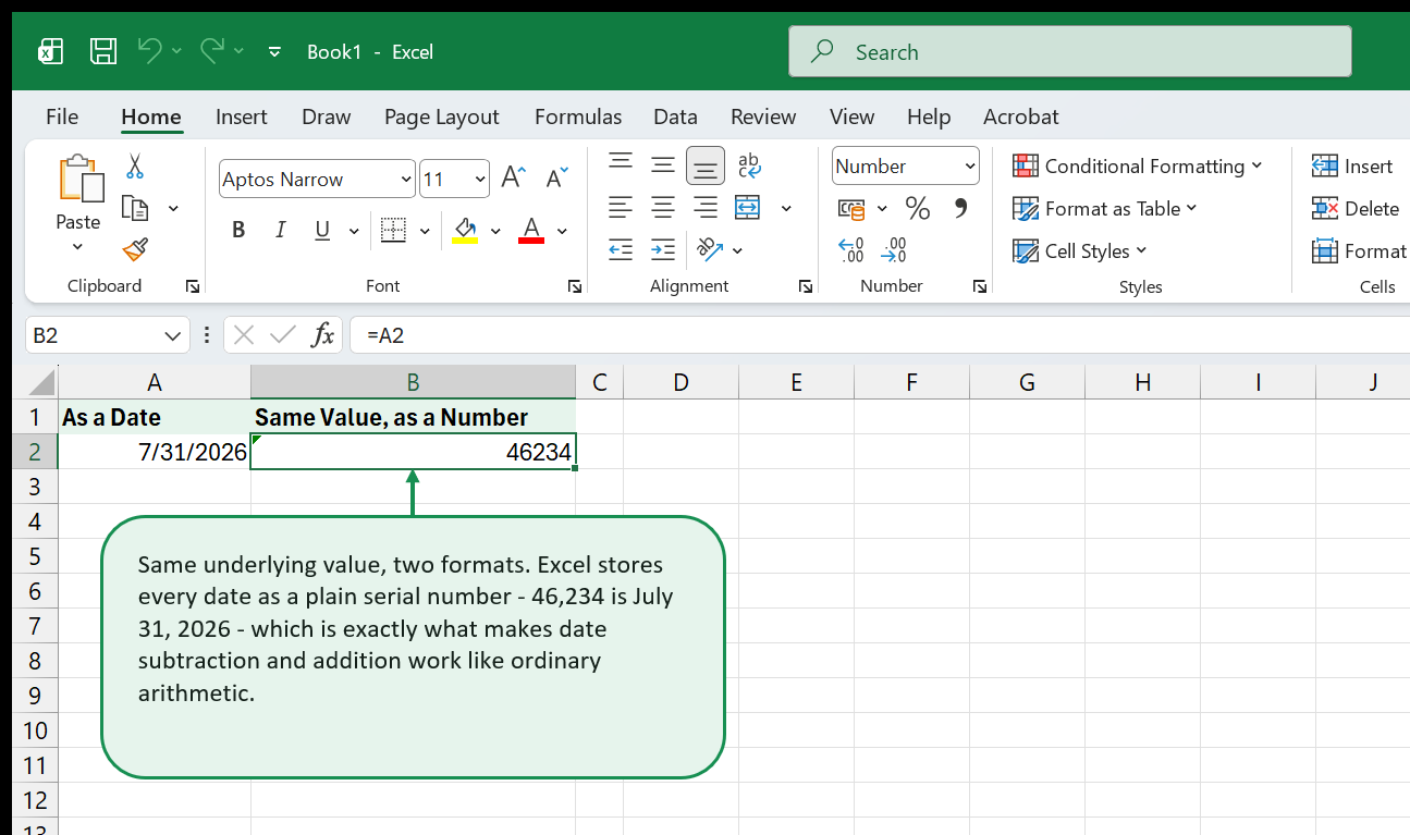
Excel does not store dates as text like “July 31, 2026.” It stores every date as a serial number — a plain integer counting the days since January 1, 1900. January 1, 1900 is serial number 1. July 31, 2026 is serial number 46,234. Times are stored as the decimal fraction of a 24-hour day: noon is 0.5, 6:00 AM is 0.25, 11:59 PM is approximately 0.9993.

This design is what makes date arithmetic so simple in Excel. To find the number of days between two dates, you just subtract one cell from the other. To add 30 days to a date, you add 30. The only complication is formatting: when Excel shows you a number where you expected a date, it means the cell is formatted as General or Number instead of Date.

Confirming a Serial Number

If you want to see the underlying serial number for any date, select the cell and change the format to Number (Home tab > Number group > dropdown). You can also use:

To convert a serial number back to a readable date, format the cell as Date or wrap it in TEXT().

The 1900 Leap Year Bug

Excel deliberately includes February 29, 1900 in its serial number sequence even though 1900 was not a leap year. This is a legacy compatibility bug inherited from Lotus 1-2-3. In practice it only matters if you are working with dates before March 1, 1900 — which is rare. For any modern date work, you will never encounter it.

---

TODAY, NOW, and Locking a Date

These two functions are the most commonly used date functions in Excel. They require no arguments and recalculate every time the workbook recalculates.

TODAY() returns a date with no time component — its decimal fraction is exactly 0. NOW() returns the current date plus the current time as a decimal. Both update automatically whenever the workbook recalculates, which means they are useful for dashboards and trackers but not for recording a fixed timestamp.

Locking a Date Permanently

If you need to stamp the current date and never have it change — a submission date, a completion date — do not use TODAY(). Instead, press Ctrl + ; (semicolon) to insert today’s date as a static value. To insert the current time as a static value, press Ctrl + Shift + ;. To insert both at once, press Ctrl + ;, then Space, then Ctrl + Shift + ;.

These shortcuts paste the literal date or time as a value, not a formula, so the cell will never change regardless of when the workbook is opened.

Using TODAY() in Calculations

Because TODAY() returns a serial number, you can use it directly in arithmetic:

This returns the number of days since the date in B2. If B2 contains a future date, the result is negative.

This returns the number of days until the date in B2 — useful for due-date countdowns.

---

Date Arithmetic: Days Between, Adding Days

The simplest date arithmetic in Excel is plain subtraction and addition. Because dates are serial numbers, these operations work exactly as expected.

Days Between Two Dates

Subtract the earlier date from the later date and you have the number of days between them. The result cell will need to be formatted as Number, not Date — Excel sometimes auto-formats subtraction results as dates, which produces confusing output like “1/30/1900.”

You can also use DAYS() for clarity:

DAYS(end, start) — note that end date comes first. The result is the same as C2-B2 but the argument order makes the intent obvious when reading a formula.

Adding and Subtracting Days

Adding or subtracting a whole number shifts the date by that many calendar days. To add weeks, multiply by 7. To add months or years, use EDATE() instead (covered in its own section) because months have different lengths.

Days vs. DATEDIF vs. NETWORKDAYS

There are three common functions for counting time between dates, and they answer different questions:

Function	Counts	Excludes weekends?	Notes
Simple subtraction / DAYS()	Calendar days	No	Fastest for raw day counts
NETWORKDAYS()	Working days	Yes	Also excludes optional holidays
DATEDIF()	Years, months, or days	No	Useful for age and tenure

---

YEAR, MONTH, DAY — Breaking Dates Apart

These three functions extract individual components from a date. They are the building blocks for grouping, filtering, and conditional logic based on dates.

All three take a single argument: a cell containing a date (or a date serial number). MONTH() returns 1 for January through 12 for December. DAY() returns the day of the month, 1 through 31.

Common Uses

To group rows by year in a pivot table, add a helper column:

To flag all rows where the month is December:

To extract the quarter from a date:

This formula converts the month number (1–12) into a quarter (1–4). It works because MONTH() returns an integer you can do arithmetic on.

---

DATE and DATEVALUE — Building Dates from Parts

If YEAR, MONTH, and DAY break dates apart, DATE and DATEVALUE put them back together.

DATE(year, month, day)

DATE() takes three numeric arguments and assembles them into a date serial number. Format the result as a Date to see it displayed properly. This is essential whenever you have year, month, and day stored in separate columns and need to combine them for sorting, filtering, or arithmetic.

This formula returns the last day of the month containing the date in B2. Adding 1 to the month and then using day 1 gives you the first day of the next month; subtracting 1 steps back to the last day of the current month. (EOMONTH() does this more directly — see its section below.)

DATE() handles out-of-range values gracefully: DATE(2026, 13, 1) rolls over to January 1, 2027, and DATE(2026, 1, 0) rolls back to December 31, 2025. This roll-over behavior is intentional and useful.

DATEVALUE(date_text)

DATEVALUE() converts a date stored as text into a date serial number. You will use this when importing data from systems that export dates as strings rather than true date values. The text must be in a format Excel recognizes — ISO 8601 (YYYY-MM-DD), US format (MM/DD/YYYY), or spelled-out formats like “July 31, 2026.”

DATEVALUE() ignores any time component in the text string. For text that includes a time, use DATEVALUE() for the date part and TIMEVALUE() for the time part, then add them.

---

WEEKDAY, WORKDAY, and NETWORKDAYS

These three functions deal with the working-week structure of a calendar — identifying day-of-week positions, projecting forward by working days, and counting working days between dates.

WEEKDAY(date, [return_type])

WEEKDAY() returns a number representing the day of the week. The second argument, return_type, controls the numbering scheme:

return_type	1 =	7 =
1 (default)	Sunday	Saturday
2	Monday	Sunday
3	0 = Monday	6 = Sunday

Using return_type 2 is the most intuitive for Monday-through-Friday workweeks. With that setting, WEEKDAY() returns 6 for Saturday and 7 for Sunday, so you can filter weekdays with:

WORKDAY(start_date, days, [holidays])

WORKDAY() projects forward (or backward, with a negative days argument) by a specified number of working days, automatically skipping Saturdays and Sundays. The optional third argument accepts a range of holiday dates to skip as well.

Where Holidays is a named range or cell reference containing a list of holiday dates.

WORKDAY.INTL() is the international variant that lets you define which days are the weekend using a weekend code or a 7-character string. Use it when your workweek is not Monday–Friday.

NETWORKDAYS(start_date, end_date, [holidays])

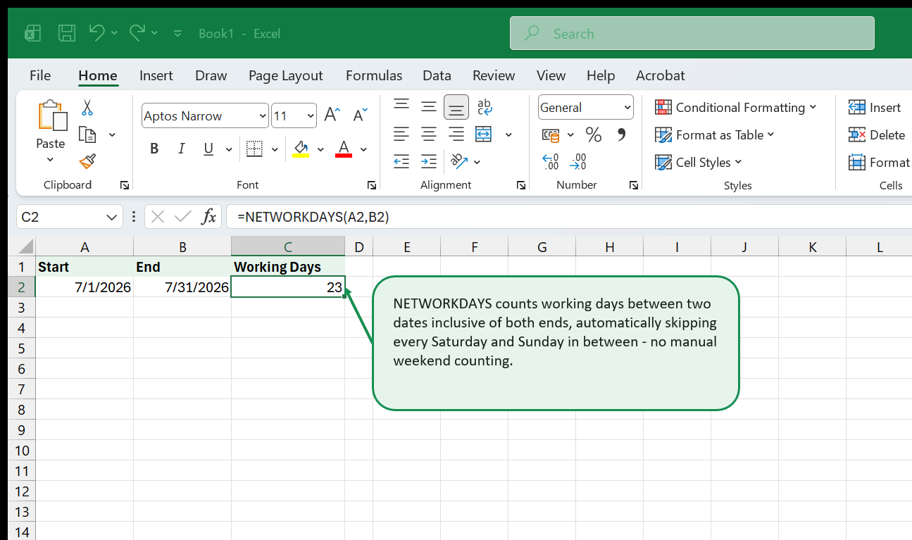
NETWORKDAYS() counts the number of working days between two dates, inclusive of both the start and end date. It automatically excludes Saturdays and Sundays. Pass a holiday range as the third argument to exclude those days too:

NETWORKDAYS.INTL() offers the same weekend customization as WORKDAY.INTL().

---

EDATE and EOMONTH

These two functions handle month-level date arithmetic — something you cannot do reliably with plain addition because months have different lengths.

EDATE(start_date, months)

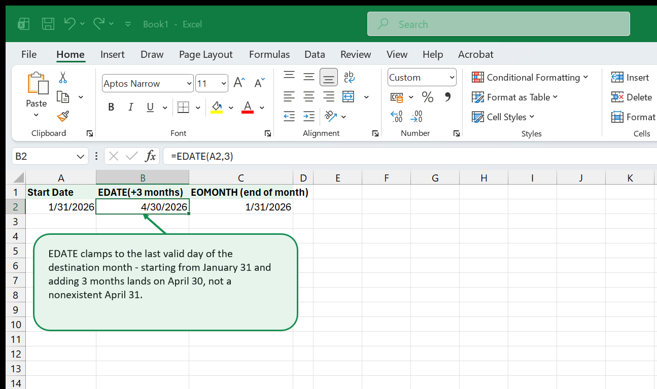
EDATE() shifts a date forward or backward by a whole number of months. A positive months argument moves forward; negative moves backward.

EDATE() preserves the day of the month where possible. EDATE(“2026-01-31”, 1) returns February 28, 2026, not March 3 — it clamps to the last valid day of the destination month. This is exactly the behavior you want for billing dates, subscription renewals, and contract terms.

EOMONTH(start_date, months)

EOMONTH() returns the last day of the month that is a specified number of months away. months=0 gives the last day of the current month. months=1 gives the last day of next month.

Adding 1 to EOMONTH(B2,0) gives the first day of the next month — a handy trick for building month-start and month-end ranges.

EOMONTH(B2,-1) is the last day of the previous month, so adding 1 gives the first day of the current month. Use this to normalize any date in a month to its month-start date.

---

HOUR, MINUTE, SECOND, and TIME

Just as YEAR, MONTH, and DAY decompose dates, HOUR, MINUTE, and SECOND decompose the time component stored in the decimal fraction of a date-time value.

These functions return integers — HOUR() from 0 to 23, MINUTE() from 0 to 59, SECOND() from 0 to 59. If B2 contains a date with no time (like a value entered with Ctrl+;), all three return 0.

TIME(hour, minute, second)

TIME() assembles a time value from its components, returning a decimal between 0 and 1. Format the result as Time to see it as a clock display. TIME() is the time equivalent of DATE().

To add 90 minutes to a time stored in B2:

To calculate elapsed time between a start time in B2 and end time in C2:

Multiplying by 24 converts the fractional day result into decimal hours. Multiply by 1440 for minutes, or by 86400 for seconds.

Handling Overnight Times

When a shift crosses midnight, simple subtraction gives a negative result. Wrap it with MOD() to handle this:

MOD(…, 1) always returns a positive fraction between 0 and 1, correctly handling the midnight rollover.

---

TEXT — Displaying Dates as Formatted Strings

TEXT() converts any value — including dates and times — into a formatted text string. It is the right tool when you need to embed a date inside a longer text string, or when you need to output a date in a specific format for export.

The second argument is a format code string — the same codes used in the Format Cells dialog (Home tab > Number group > More Number Formats). Common date codes:

Code	Output for July 31, 2026
D	31
DD	31
DDD	Fri
DDDD	Friday
M	7
MM	07
MMM	Jul
MMMM	July
YY	26
YYYY	2026

Concatenating Dates into Sentences

A common use case is building dynamic labels:

Without TEXT(), concatenating a date with & would produce its serial number rather than a readable date string.

---

DATEDIF — Age and Tenure Calculations

DATEDIF is one of Excel’s most useful date functions and one of its least documented. It does not appear in Excel’s formula autocomplete list, and it is not in the official function reference — it survives from Lotus 1-2-3 compatibility. Despite this, it works correctly in all modern Excel versions and Microsoft 365.

Syntax: =DATEDIF(start_date, end_date, unit)

The unit argument controls what DATEDIF counts:

Unit	Returns
“Y”	Complete years between dates
“M”	Complete months between dates
“D”	Days between dates (same as subtraction)
“MD”	Days remaining after subtracting complete months
“YM”	Months remaining after subtracting complete years
“YD”	Days remaining after subtracting complete years

Calculating Age

This returns a person’s age in complete years. Unlike dividing by 365, it correctly handles leap years and gives you an integer — not a decimal.

Full Age String (Years, Months, Days)

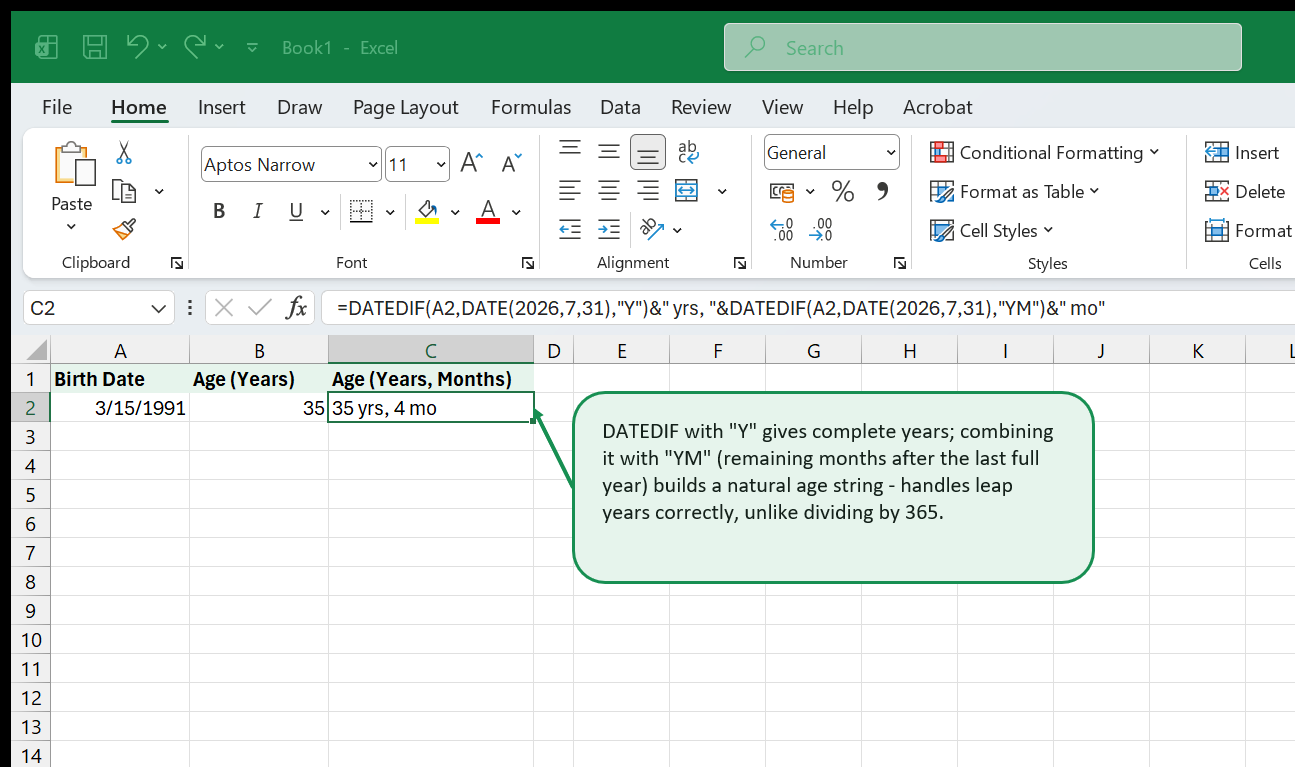
Combining “Y” and “YM” gives you the age in years and the remaining months — useful for HR profiles, loan applications, or patient records.

Employee Tenure

DATEDIF(start, end, “M”) gives you the total months of tenure as a plain integer, which is useful for tier-based benefits calculations.

DATEDIF Gotcha

DATEDIF requires start_date to be earlier than end_date. If start is later than end, it returns a #NUM! error rather than a negative number. Wrap with IFERROR() if your data might contain future start dates:

---

Common Patterns

Project Deadline Status Flag

Flag each task row as Overdue, Due Today, Due Soon (within 7 days), or On Track:

Assign conditional formatting rules on this column using the cell value equal to “Overdue” (red), “Due Today” (orange), and “Due Soon” (yellow) to create a visual traffic-light tracker.

Days Until Deadline (Negative = Past Due)

Format the column as Number. Negative values mean the deadline has passed. Sort ascending to surface the most overdue items at the top.

Working Days Until Deadline

Subtracting 1 excludes today from the count, giving you the number of full working days remaining. Add the Holidays range as a third argument if you track company holidays.

Age Bin (for Segmentation)

IFS() (available in Excel 2019 and Microsoft 365) chains conditions cleanly. Use nested IF() for earlier Excel versions.

Month-Over-Month Comparison Key

To join two tables on year-month (e.g., actuals vs. budget), create a consistent key column:

This produces an integer like 202607 that sorts and matches correctly across tables without any text formatting quirks.

First and Last Day of a Fiscal Quarter

Assuming fiscal year starts in April (Q1 = Apr–Jun):

Adjust the month offset to match your fiscal year start.

---

Quick Reference Table

Function	Syntax	Returns	Example
TODAY	=TODAY()	Today’s date	7/31/2026
NOW	=NOW()	Current date and time	7/31/2026 14:35
DATE	=DATE(year, month, day)	Date serial number	=DATE(2026,7,31)
DATEVALUE	=DATEVALUE(text)	Date serial from text	=DATEVALUE(“2026-07-31”)
YEAR	=YEAR(date)	Year integer	2026
MONTH	=MONTH(date)	Month integer (1–12)	7
DAY	=DAY(date)	Day of month (1–31)	31
DAYS	=DAYS(end, start)	Calendar days between	=DAYS(C2,B2)
WEEKDAY	=WEEKDAY(date, [type])	Day-of-week number	=WEEKDAY(B2,2)
WORKDAY	=WORKDAY(start, days, [holidays])	Date N working days away	=WORKDAY(B2,10)
WORKDAY.INTL	=WORKDAY.INTL(start, days, weekend, [holidays])	Date N working days away (custom weekend)	=WORKDAY.INTL(B2,10,2)
NETWORKDAYS	=NETWORKDAYS(start, end, [holidays])	Working days between dates	=NETWORKDAYS(B2,C2)
NETWORKDAYS.INTL	=NETWORKDAYS.INTL(start, end, weekend, [holidays])	Working days (custom weekend)	=NETWORKDAYS.INTL(B2,C2,2)
EDATE	=EDATE(start, months)	Date N months away	=EDATE(B2,3)
EOMONTH	=EOMONTH(start, months)	Last day of month N months away	=EOMONTH(B2,0)
DATEDIF	=DATEDIF(start, end, unit)	Difference in Y/M/D units	=DATEDIF(B2,TODAY(),“Y”)
TEXT	=TEXT(value, format_text)	Formatted date string	=TEXT(B2,“MMM YYYY”)
HOUR	=HOUR(time)	Hour (0–23)	=HOUR(B2)
MINUTE	=MINUTE(time)	Minute (0–59)	=MINUTE(B2)
SECOND	=SECOND(time)	Second (0–59)	=SECOND(B2)
TIME	=TIME(hour, minute, second)	Time decimal fraction	=TIME(14,30,0)
TIMEVALUE	=TIMEVALUE(text)	Time decimal from text	=TIMEVALUE(“2:30 PM”)
ISOWEEKNUM	=ISOWEEKNUM(date)	ISO week number (1–53)	=ISOWEEKNUM(B2)
WEEKNUM	=WEEKNUM(date, [type])	Week number of year	=WEEKNUM(B2,2)

---

Where to Go Next

Date and time functions become even more powerful when you combine them with lookup, conditional, and aggregation functions. These guides cover the next logical steps:

• XLOOKUP & VLOOKUP Field Guide — use XLOOKUP to pull schedule data, map date ranges to categories, and join tables by a date key.
• IF — build overdue flags, status labels, and conditional date logic with IF, AND, and OR.
• Pivot Tables from Zero — group date fields by week, month, quarter, and year automatically inside PivotTables, no helper columns required.
• LAMBDA & Dynamic Arrays — use FILTER and SORT with date conditions to build self-updating calendars and schedule views.
• Conditional Formatting Mastery — apply color scales, icon sets, and formula-based rules to highlight deadlines, overdue rows, and date ranges visually.

Want to practice on a larger, realistic dataset? Download the PivotTable practice: sales transactions dataset - 300 rows with a real date column, ready for EOMONTH grouping, NETWORKDAYS turnaround calculations, or a YEAR/MONTH key of your own.