LAMBDA & Dynamic Arrays

Excel changed fundamentally in 2019 when Microsoft introduced dynamic arrays. Before that, getting a formula to return multiple values required pressing Ctrl+Shift+Enter and hoping the result landed in exactly the right number of cells. Today, a single formula can spill an entire filtered, sorted, deduplicated table into a worksheet with no special handling required. If you have been building complex nested IF statements and multi-step VLOOKUP chains, this ebook will show you a cleaner way to work.

This guide is for Excel users who already know their way around common lookup and reference functions. You should be comfortable with XLOOKUP or VLOOKUP, understand how relative and absolute cell references work, and have used at least a few IF-based formulas. What you may not have explored yet is the dynamic array engine — FILTER, SORT, UNIQUE, SEQUENCE — and the two functions that sit above all of them: LET, which lets you name intermediate calculations inside a formula, and LAMBDA, which lets you define entirely new functions that live in your workbook.

Work through the chapters in order the first time. The later sections on LAMBDA, MAP, and REDUCE build directly on the dynamic array concepts introduced earlier, and the real-world use cases in Chapter 10 pull every technique together into patterns you can copy straight into your own files. All formulas in this ebook assume Excel 365 or Excel 2021. If a function does not appear on your version, check whether your organisation’s Microsoft 365 channel is set to Current Channel, which receives new features first.

The Dynamic Array Revolution

Dynamic arrays are not just new functions — they represent a new calculation model. Any formula that returns more than one value now automatically spills those values into adjacent cells, expanding as far as necessary. This single change makes an enormous number of previously awkward formulas straightforward.

The Spill Range and the # Operator

When a dynamic array formula runs, Excel places the top-left result in the formula cell and fills the remaining values into the cells below or to the right. That occupied region is called the spill range. If anything blocks the spill — another value, a merged cell, even a space character — Excel shows a #SPILL! error until the obstruction is cleared.

The hash operator (#) lets you reference an entire spill range by pointing at just the formula cell. Suppose a UNIQUE formula in D2 spills ten distinct values into D2:D11. Any other formula can reference the whole list as D2# rather than D2:D11, and if the list grows or shrinks, D2# updates automatically.

The formula above spills every distinct value from column B into consecutive cells. Anywhere else in the sheet, reference the result with:

That count adjusts the moment the source data changes — no manual range adjustment needed.

Legacy Ctrl+Shift+Enter Arrays

Before dynamic arrays, power users pressed Ctrl+Shift+Enter to create what are sometimes called CSE arrays or legacy arrays. You will still encounter these in older workbooks, wrapped in curly braces: {=SUM(IF(B2:B20>100,C2:C20,0))}. Dynamic arrays make most CSE arrays unnecessary, and mixing the two styles in one formula is rarely worthwhile. When you find a CSE array that a dynamic function can replace, rewrite it — the modern version will be easier to maintain and will not confuse colleagues who have never seen curly-brace formulas.

FILTER — Extracting Conditional Subsets

FILTER is the function that replaces the most common reason people used to reach for Advanced Filter or a macro. It returns every row from a range that meets one or more criteria, and the result updates automatically when the source data changes.

Basic Syntax

=FILTER(array, include, [if_empty])

• array — the range of data you want to return (can be multiple columns)
• include — a TRUE/FALSE array the same height as array; rows where this is TRUE are returned
• if_empty — optional; what to show if nothing matches (without this, FILTER returns #CALC! when no rows pass)

That formula returns every row from A2:C20 where column B exceeds 100. Add the third argument so the cell does not sit blank when the filter finds nothing.

Multiple Conditions

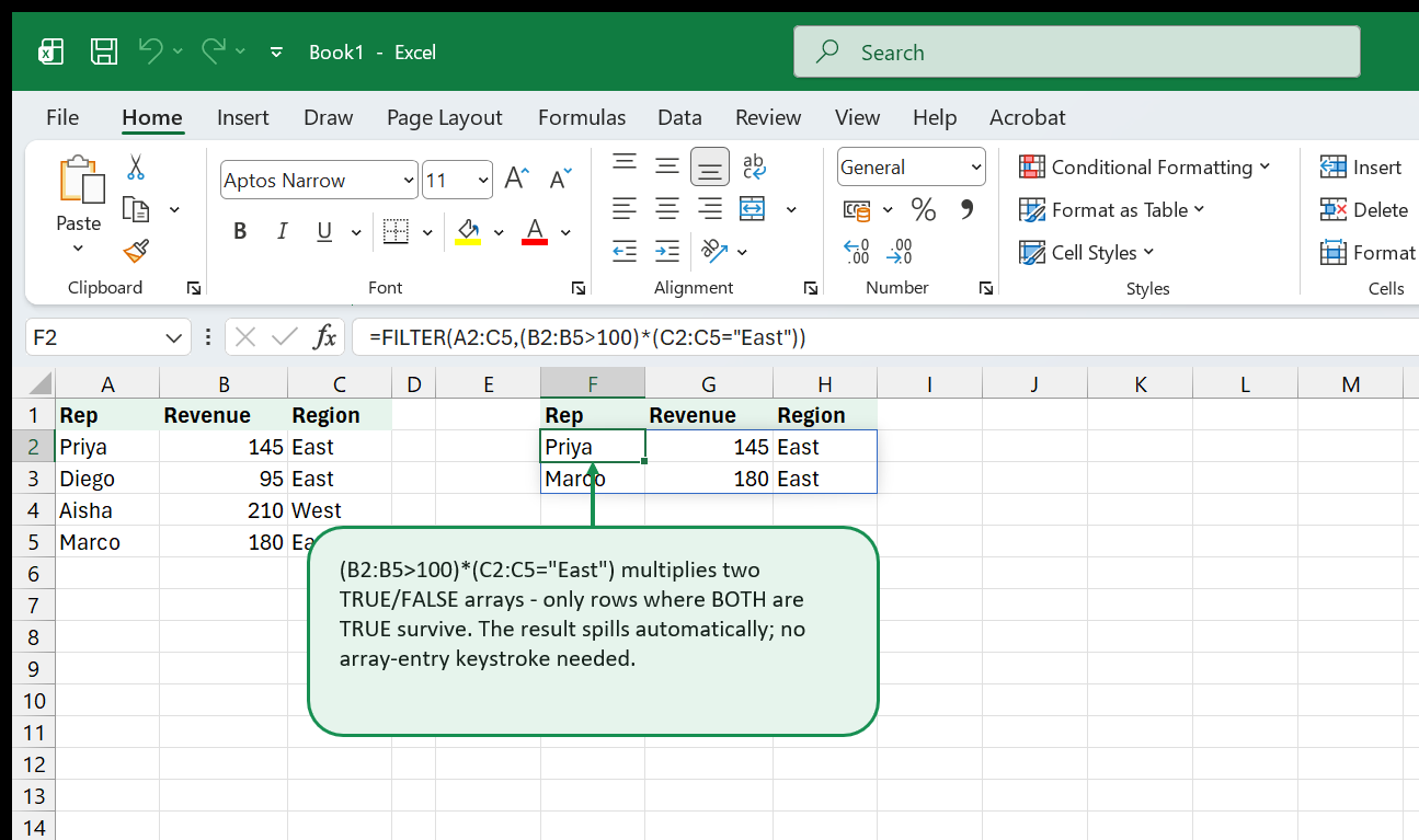
Combine conditions with multiplication for AND logic and addition for OR logic. Multiplication works because TRUE is 1 and FALSE is 0 — multiplying two TRUE/FALSE arrays gives 1 only when both are TRUE.

For OR logic, use addition and wrap in a double negative or comparison to convert to TRUE/FALSE:

Any row where either condition is true has a sum of at least 1, which FILTER treats as TRUE.

FILTER with a Partial Match

ISNUMBER combined with SEARCH gives you a contains-style text filter:

SEARCH is case-insensitive; swap it for FIND if case matters.

SORT and SORTBY — Ordered Results on the Fly

Sorting a range used to mean selecting it, running Data > Sort, and repeating whenever the data changed. SORT and SORTBY return a sorted copy of a range as a formula result, leaving the source unchanged.

SORT

=SORT(array, [sort_index], [sort_order], [by_col])

• sort_index — which column (or row) to sort by; defaults to 1
• sort_order — 1 for ascending (default), -1 for descending
• by_col — FALSE to sort rows (default), TRUE to sort columns

This returns A2:C20 sorted by the second column, largest to smallest.

SORTBY

SORTBY is more flexible: the column you sort by does not have to be in the returned array, and you can chain multiple sort levels.

=SORTBY(array, by_array1, [sort_order1], [by_array2], [sort_order2], ...)

That returns column A, sorted first by column B descending, then by column C ascending — a two-level sort in a single formula.

Sorting a FILTER Result

Because dynamic array functions return arrays, they chain naturally:

One formula: filter to the West region, sort the result by the second column descending. No helper columns, no intermediate tables.

UNIQUE — Deduplicating Lists Automatically

UNIQUE extracts distinct values from a list or range, updating automatically as the source changes. It is the formula equivalent of Data > Remove Duplicates, but non-destructive — the source data stays intact.

Basic Syntax

=UNIQUE(array, [by_col], [exactly_once])

• by_col — FALSE returns unique rows (default), TRUE returns unique columns
• exactly_once — FALSE returns each distinct value once (default), TRUE returns only values that appear exactly once

The second example returns unique rows across all three columns — a row is only included if no other row has the same combination in columns A, B, and C.

UNIQUE + SORT for Clean Drop-Down Lists

Combining UNIQUE and SORT is the standard recipe for a self-updating source list for data validation drop-downs, covered in detail in Chapter 10.

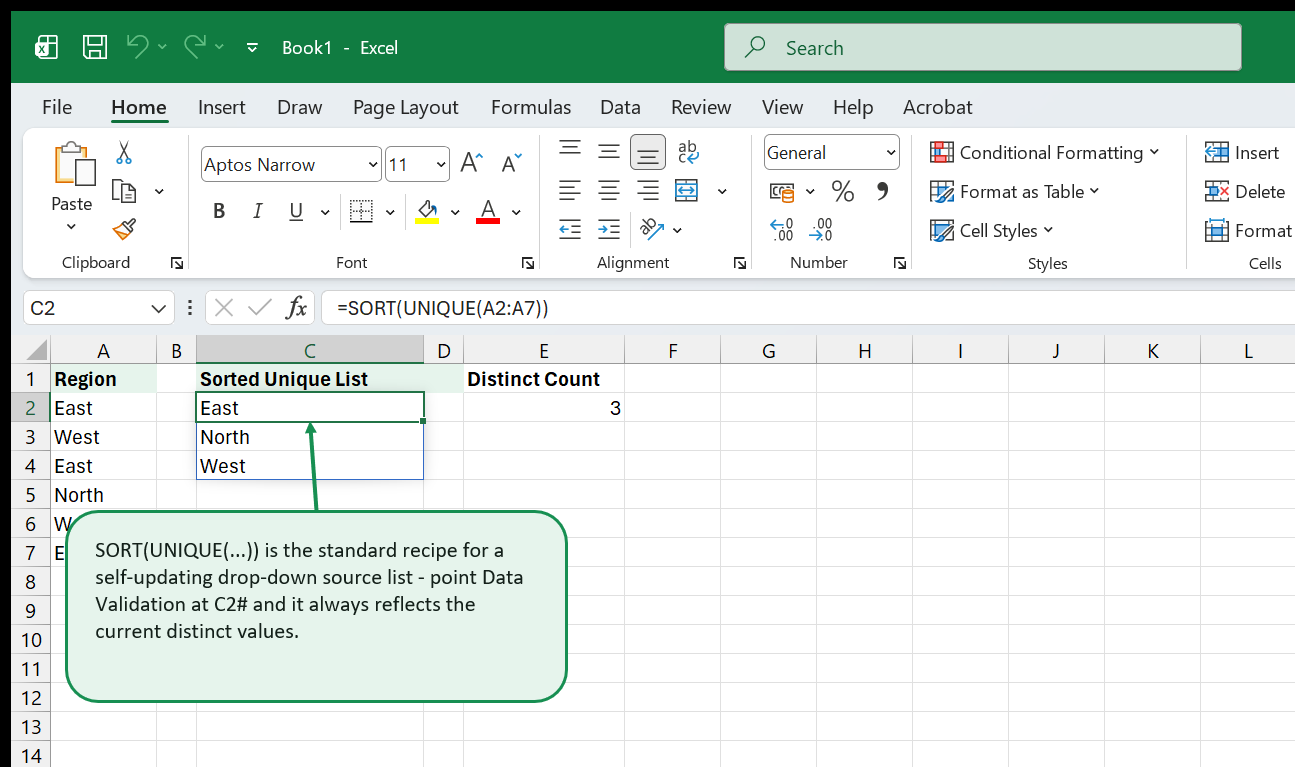
Counting Distinct Items

Wrap UNIQUE in COUNTA to count how many distinct values exist:

SEQUENCE — Generating Number and Date Series

SEQUENCE fills a range with a series of numbers, which you can shape into rows, columns, or grids and shift by any start value and step.

Basic Syntax

=SEQUENCE(rows, [cols], [start], [step])

Argument	Default	Meaning
rows	required	number of rows in the output
cols	1	number of columns
start	1	first value
step	1	increment between values

Returns 1, 2, 3 … 10 in a single column.

Returns a 5-row by 4-column grid starting at 0, incrementing by 5: 0, 5, 10, 15 across the first row, 20, 25, 30, 35 across the second, and so on.

Date Series with SEQUENCE

Because Excel dates are serial numbers, SEQUENCE generates date ranges directly:

That produces twelve dates spaced thirty days apart starting 1 January 2026 — a quick way to build a monthly schedule header.

For the first day of each month specifically, wrap with EOMONTH:

Row Numbers for Formulas

SEQUENCE(ROWS(A2:A100)) generates a helper column of row offsets without occupying a real column, useful inside INDEX-based constructions where you previously would have dragged down a 1, 2, 3 series.

Combining Dynamic Array Functions

The real power comes from nesting these functions. Each returns an array, so the output of one is a valid input to another.

Ranked Unique List

Extract distinct values and rank them by a related metric in one step:

UNIQUE pulls the distinct items; COUNTIF counts how many times each appears in the original range; SORTBY arranges the unique list by those counts, highest first. The result is a frequency-ranked list with no pivot table required.

Filtered and Sorted Multi-Column Output

Returns all closed deals worth more than 10 000, sorted by the value column (column 4) from largest to smallest.

SEQUENCE Inside INDEX

A common pattern before dynamic arrays was to drag INDEX down a column to pick different rows. SEQUENCE replaces the drag:

That starts from the row of the maximum value and returns five consecutive names — useful for extracting a top-N block when you already know the position.

LET — Naming Formula Steps for Clarity

LET solves a problem every formula writer eventually hits: you need the same sub-calculation in three places inside one formula, so you either repeat it three times (making the formula fragile) or introduce a helper cell (breaking the single-formula approach). LET gives you named variables inside a formula.

Basic Syntax

=LET(name1, value1, [name2, value2, ...], calculation)

You define pairs of name and value, then the final argument is the expression that uses those names.

Here sales and target are calculated once and reused in the FILTER. With long ranges or complex sub-expressions, this makes formulas dramatically easier to read and modify.

A Practical LET Example

Without LET, a bonus calculation that references the same adjusted-salary expression three times looks like this:

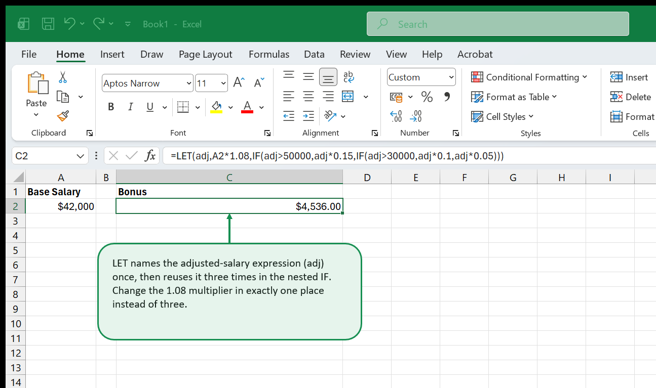
=IF((B2*1.08)>50000, (B2*1.08)*0.15, IF((B2*1.08)>30000, (B2*1.08)*0.10, (B2*1.08)*0.05))

With LET:

The adjusted salary is computed once. If the 1.08 multiplier changes, you update it in one place.

LET with Dynamic Arrays

LET works naturally with array-returning functions. Naming an intermediate filtered result and then sorting it reads much more clearly than nesting SORT directly inside FILTER:

Name the filtered set, then sort it. Each step is readable on its own.

LAMBDA — Writing Your Own Excel Functions

LAMBDA is the most significant addition to the Excel formula language in decades. It lets you define a reusable custom function — with named parameters — entirely inside a formula. Once saved to Name Manager, your LAMBDA function works exactly like a built-in function across the entire workbook.

Basic Syntax

=LAMBDA(param1, [param2, ...], calculation)

Typed directly in a cell, a LAMBDA does nothing until you call it by appending parentheses with arguments:

That calls an anonymous squaring function with 5 as the argument. Anonymous LAMBDA calls are useful for testing, but the real value comes from storing them in Name Manager.

Creating a Named LAMBDA Function

1. Open Formulas tab > Name Manager > New.
2. Give the name something descriptive, such as TAXRATE.
3. In the Refers To box, enter the LAMBDA formula — no leading = is required by some versions, but include it to be safe:

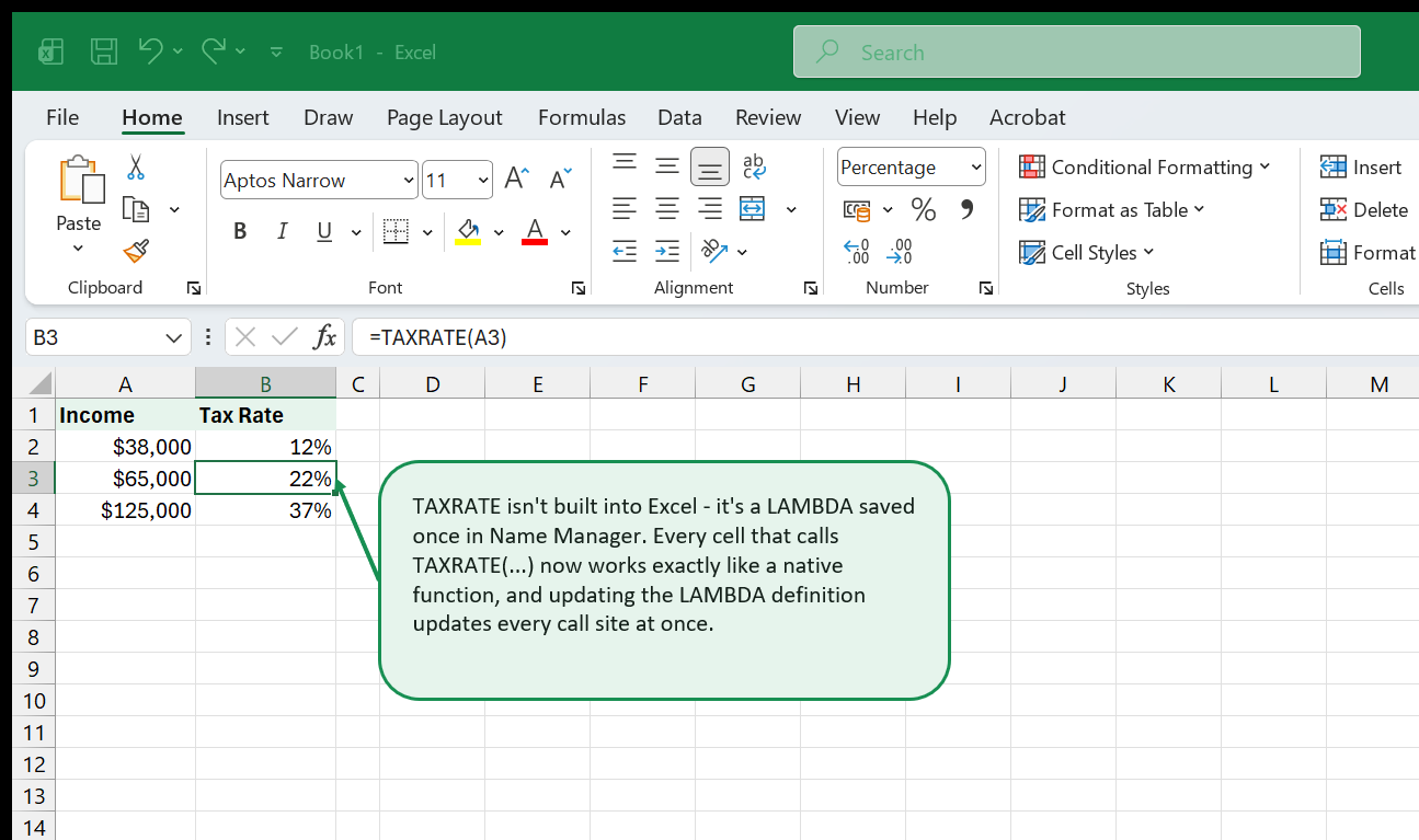
=LAMBDA(income, IF(income>100000, 0.37, IF(income>44725, 0.22, 0.12)))

4. Click OK.

Now anywhere in the workbook you can write:

Change the brackets in Name Manager once and every cell using TAXRATE updates.

Recursive LAMBDA

LAMBDA supports recursion via a second optional name argument. The pattern is to give the LAMBDA its own name as a parameter so it can call itself:

=LAMBDA(FACTORIAL, n, IF(n<=1, 1, n * FACTORIAL(FACTORIAL, n-1)))

Store this as FACTORIAL in Name Manager, then call it:

Recursive LAMBDA is advanced territory — most workbook problems do not need it — but it removes the last category of things that genuinely required VBA for formula-only work.

LAMBDA Best Practices

Keep each LAMBDA focused on one transformation. If a function needs ten parameters, it is almost always clearer to break it into two or three named LAMBDAs that call each other. Document the parameter names carefully in the Name Manager Comment field — your future self will thank you when the workbook reappears six months later.

MAP, REDUCE, BYROW, BYCOL

These four functions apply a LAMBDA to every element of an array, or accumulate an array down to a single value. They arrive as a group and are designed to be used with LAMBDA.

MAP

MAP applies a LAMBDA to every element of one or more arrays and returns an array of the same shape.

=MAP(array1, [array2, ...], lambda)

Returns every value in A2:A20 increased by ten percent. This is equivalent to =A2:A20*1.1 for simple arithmetic, but MAP becomes valuable when the per-element logic involves a named LAMBDA that encapsulates complexity.

With two arrays, MAP passes one element from each to the LAMBDA simultaneously:

Element-wise multiplication of two columns — similar to =B2:B20*C2:C20 but named and explicit.

REDUCE

REDUCE accumulates an array into a single value by applying a LAMBDA repeatedly. The LAMBDA receives the running accumulator and the current element.

=REDUCE([initial_value], array, lambda)

This is equivalent to SUM, but REDUCE handles accumulations that no built-in function covers directly. For example, a running product:

BYROW and BYCOL

BYROW and BYCOL apply a LAMBDA to each row or each column of a range and return an array of one result per row or column.

=BYROW(array, lambda)
=BYCOL(array, lambda)

Returns the maximum value in each row across four columns — a 19-value column of row maxima. Previously this required either MAX with IF as a CSE array or a helper column.

Returns four values — the average of each column. A column of averages without a SUBTOTAL or a separate AVERAGE row.

Combining MAP and LAMBDA

The real benefit of MAP is pairing it with a named LAMBDA. If TAXRATE is already defined in Name Manager:

Apply your custom function to every row in one formula. When the tax logic changes, update TAXRATE once.

Real-World Use Cases

Dynamic Dependent Drop-Downs

Standard data validation drop-downs require a fixed range. With UNIQUE and SORT producing a spill range, you can point a drop-down at D2# and it will always contain the current distinct values from your source column.

Step 1: In D2, build the master unique list:

Step 2: In a second helper column, say F2, build a filtered list for a dependent drop-down. If the first drop-down selection lands in H1:

Step 3: Select the cells where the dependent drop-down should appear. Go to Data tab > Data Validation > Allow: List. In the Source box, type =$F$2#. Excel accepts the spill reference and the list grows or shrinks as H1 changes.

This technique replaces the traditional approach of building a named range for every possible parent value — a maintenance nightmare on large datasets.

Auto-Ranked Leaderboard

A leaderboard that stays correct without sorting the source data and without a pivot table:

Source data: Names in column A, scores in column B, region in column C.

Leaderboard formula (paste into E2):

That returns the North region rows sorted by score, descending. Wrap the whole thing in TAKE to limit to top five:

TAKE(array, rows) returns the first N rows — available in Excel 365 from late 2022 onward. If TAKE is not available on your version, wrap the SORTBY in INDEX with SEQUENCE(5) to achieve the same top-five result:

Building a Reusable AVERAGEIF-Style LAMBDA

Excel has AVERAGEIF, but no AVERAGEIFS-equivalent that handles arrays gracefully. A LAMBDA covers the gap:

In Name Manager, define AVGIF as:

=LAMBDA(range, criteria_range, criteria,
    AVERAGE(IF(criteria_range=criteria, range)))

Call it:

Any time the filter logic becomes more complex — say, criteria drawn from a spill range — the LAMBDA body handles it and every call site stays clean.

Month-Over-Month Summary with SEQUENCE and SUMIFS

Generate a summary table of monthly totals without a pivot table:

In G2, place the month start dates:

In H2, reference the spill range to sum each month:

One formula in H2 produces twelve monthly totals aligned with the dates in G2. Add new transactions to columns B and C and both columns update instantly.

Where to Go Next

The functions in this ebook form the productive core of modern Excel formula writing, but they connect to broader skills. The resources below will help you apply what you have learned:

• Excel Formulas Cheat Sheet — a quick-reference companion covering the essential functions LAMBDA and dynamic arrays rely on, including TEXT, DATE, and logical functions
• Excel Intermediate Skills — if any section in this ebook felt like a stretch, that guide fills the gaps with named ranges, data validation, and structured table references
• Microsoft’s official Excel function reference — the authoritative syntax reference for every function covered here, including argument constraints and version availability notes
• The Name Manager (Formulas tab > Name Manager) — your LAMBDA library lives here; take time to document each entry with a comment explaining parameters and purpose before sharing the workbook
• Excel’s Trace Dependents and Evaluate Formula tools (Formulas tab > Formula Auditing) — essential for debugging nested dynamic array formulas when a result looks wrong; Evaluate Formula steps through the calculation in sequence, showing the intermediate array at each stage

Want a bigger dataset to practice FILTER, SORT, and UNIQUE on? Download the SUMIFS / COUNTIFS practice dataset - 200 rows across region, product, month, and salesperson, plenty of real structure for multi-condition FILTER formulas and ranked UNIQUE lists.