
Chapter 1: The Mindset of Calm Formula Debugging
Seeing a wall of #N/A, #REF!, or #SPILL! across an executive summary ten minutes before a deadline feels stressful—until you realize Excel error codes are not random failures. Every single Excel error badge tells you which step of evaluation stopped and why.
Panic debugging makes workbooks worse. Copying values over broken cells destroys traceability, wrapping an entire sheet in IFERROR(..., 0) hides genuine data loss behind reassuring zeros, and guessing fixes without checking precedent cells creates circular loops.
Professional spreadsheet auditors work top-down using three disciplined rules:
- Find the origin error, not the echo: When a single
#DIV/0!cell feedsSUM(), twelve downstream KPIs turn#DIV/0!. Always trace back to the earliest broken input cell first. - Inspect stored values, never formatted appearances: A cell formatted as
"$3.33"may store3.334, and a cell displaying"SKU-102"may hold"SKU-102 "with an invisible trailing space. - Fix root data types rather than masking errors: Clean text coercion, explicit zero denominators, and structured ranges prevent repeat failures permanently.
Chapter 2: Excel’s Built-In Auditing Toolkit
Before editing a single formula bar character, master the four native inspection tools under the Formulas ribbon tab (Formula Auditing group):
| Auditing Tool | Shortcut | What It Reveals Immediately |
|---|---|---|
| Trace Precedents | Alt + M + P |
Draws blue arrows from every input cell feeding the active formula |
| Trace Dependents | Alt + M + D |
Shows every downstream KPI or sheet impacted if you edit this cell |
| Evaluate Formula | Alt + M + V |
Steps through nested parentheses one evaluation click at a time |
| Watch Window | Formulas -> Watch Window | Pins distant summary totals visibly while you fix raw data on another tab |
The Partial Selection F9 Trick
Inside the formula bar, highlight any self-contained sub-expression (such as TRIM(A3) or C2:C10>0) and press F9. Excel evaluates only the highlighted segment right inside the formula bar so you can verify intermediate arrays instantly. Always press Esc afterward (never Enter) so you do not overwrite your dynamic formula with static preview values!
Chapter 3: Cracking #N/A Lookup Failures
#N/A stands for “Not Available” and appears almost exclusively inside lookup and matching functions (VLOOKUP, XLOOKUP, INDEX/MATCH, XMATCH). More than 70% of #N/A errors occur even when the eye sees identical words in both columns—because computers match exact character bytes and data types, not visual similarity.
Four Hidden Causes of False #N/A Matches
- Trailing spaces (
"SKU-102 "vs"SKU-102"): Imported ERP exports love padding right-hand spaces. - Non-breaking spaces (
CHAR(160)): Copied HTML tables contain web characters that standardTRIM()ignores! - Text vs Numeric IDs (
"00412"vs412): Leading zeros turn IDs into text in one table while the other parsed integers. - Missing 4th match-mode or fallback argument: Legacy
VLOOKUPwithoutFALSEfails silently or returns the wrong row; omission inXLOOKUPlets raw#N/Aleak into downstreamSUM.
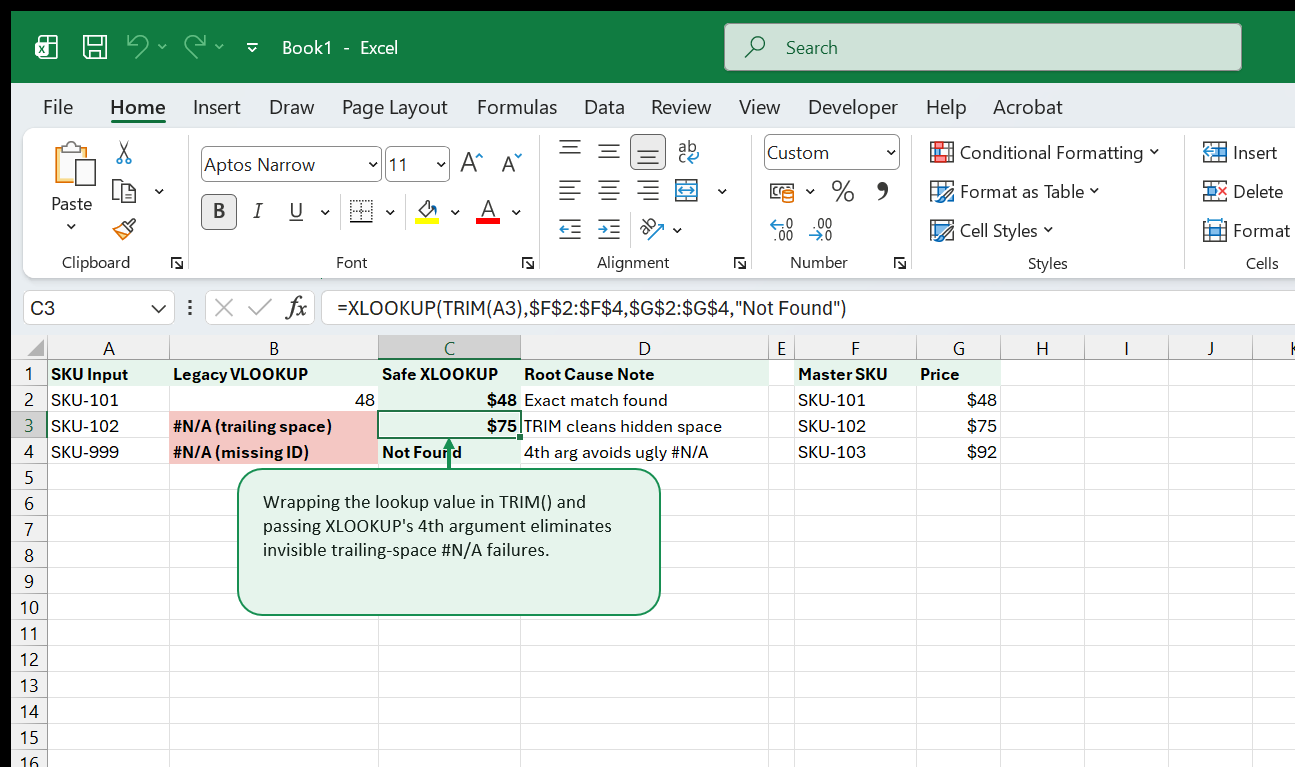
Surgical Fix Pattern
Strip both standard whitespace and HTML non-breaking spaces before matching:
=XLOOKUP(TRIM(SUBSTITUTE(A3,CHAR(160)," ")), Master!$F$2:$F$4, Master!$G$2:$G$4, "Not Found")Notice that using "Not Found" explicitly tells auditors why SKU-999 returned empty without poisoning numeric SUM() aggregations (remember SUM() ignores text cleanly, whereas #N/A breaks SUM()!).
Chapter 4: Resolving #SPILL! Dynamic Array Conflicts
#SPILL! arrived with Excel’s dynamic array engine (UNIQUE, FILTER, SORT, SEQUENCE, XLOOKUP returning multiple columns). When a dynamic formula wants to output 3 rows vertically (C2:C4), every single target cell below C2 must be completely empty.
If even one stray spacebar character, leftover comment note, or merged box sits inside the spill zone, Excel refuses to overwrite existing content and raises #SPILL!.
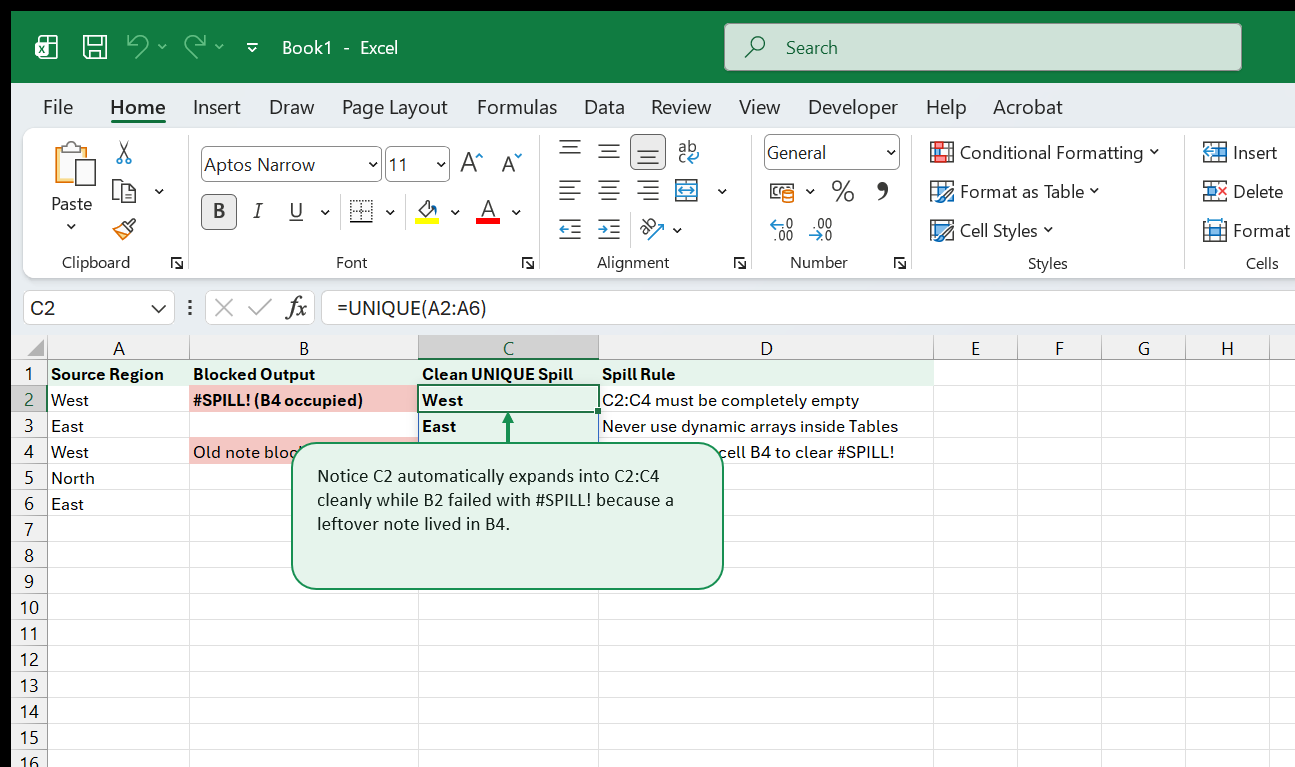
Five Ways to Fix #SPILL! in Seconds
- Click the floating warning icon -> Select Obstructing Cells: Excel jumps the cursor directly onto
B4so you can inspect or clear the blocker. - Unmerge cells: Merged cells inside a spill zone block dynamic expansion every time.
- Move formulas out of Excel Tables: Formal
Ctrl+TTables do not permit multi-cell spilling inside a single table column! Either wrap the formula inside single-row scalars (@), convert the range back to a normal range, or place dashboardFILTER/UNIQUEtables outside Tables. - Watch invisible
""formula strings: Another formula returning empty string""looks blank visually, yet occupies the cell and blocks spills!
Chapter 5: Fixing #VALUE! Type Mismatches and Hidden Text
#VALUE! tells you an operator (+, -, *, /) or strict function received the wrong data type—most commonly trying to multiply text like "$1,250.00" (or " 450 " containing spaces or European commas) by a numeric quantity.
Ironically, =SUM(A2:A4) silently skips text cells with zero error warning, whereas =A2+A3 crashes immediately with #VALUE!. That mismatch fools millions of analysts when totals suddenly disagree!
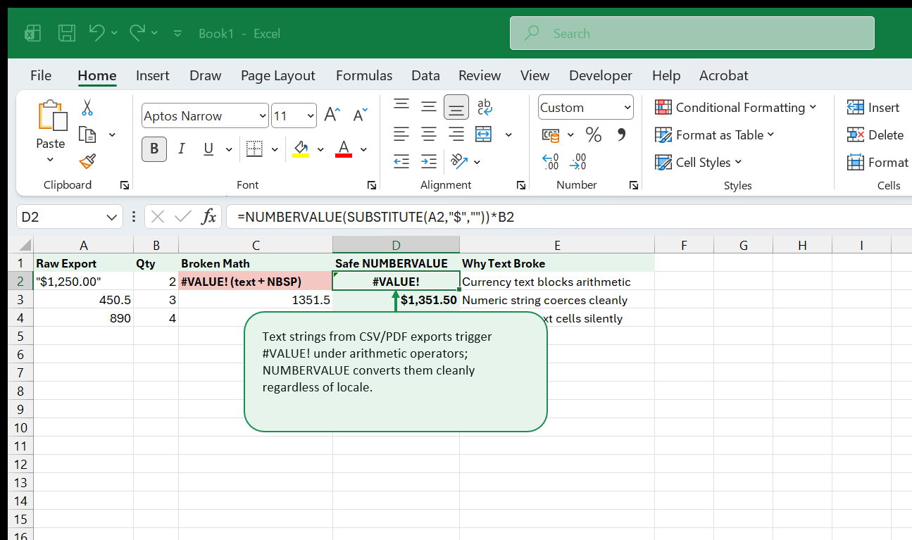
Universal Text-to-Number Repair Chain
Use NUMBERVALUE() whenever international decimal/thousand separators (1.250,00 vs 1,250.00) mix inside exports:
=NUMBERVALUE(SUBSTITUTE(SUBSTITUTE(A2,"$",""),CHAR(160),""))*B2Chapter 6: Eliminating #REF! Broken Link Disasters
#REF! stands for Invalid Reference. Once a formula cell displays #REF!, Excel has already forgotten what coordinate lived there before the break! That makes #REF! the most destructive error in financial models because Undo (Ctrl+Z) or backup comparison is sometimes required if you did not inspect the break right away.
Common causes:
- Deleting a worksheet, column, or row that another sheet pointed to directly.
- Writing
OFFSETorINDEXbeyond array boundaries (for example,INDEX(B2:C2, 1, 5)). - Pasting shifted ranges over active referenced headers.
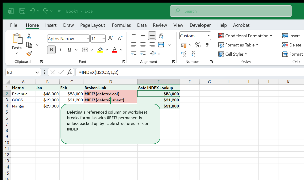
Defensive Habits Against #REF!
- Before deleting ANY column or tab, press Ctrl+F (
Look in: Formulas) or click Trace Dependents across the candidate range so hidden cross-sheet consumers show themselves first. - Prefer Excel Table Column Names (
tblSales[Revenue]): Moving columns or inserting rows never corrupts named Table columns—and even clearing rows preserves structural formulas cleanly. - Hide or archive retired input columns gently during close weeks instead of deleting structure while downstream dashboards still depend on it.
Chapter 7: Guarding #DIV/0! Without Blind IFERROR Masking
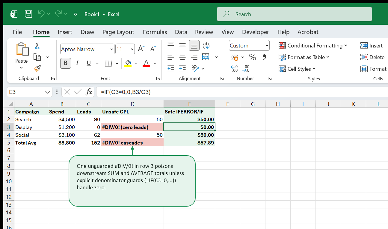
Dividing any number by zero or an empty cell emits #DIV/0!. While tempting to blanket every sheet in =IFERROR(B2/C2, 0), blind IFERROR masking swallows #REF!, #NAME?, and #N/A bugs right alongside zero denominators—turning real structural damage into innocent-looking zeros!
Always reserve your guard specifically for the expected zero denominator condition:
=IF(C3=0, 0, B3/C3)Or in Excel 365/2024 Power Pivot DAX, DIVIDE([Spend], [Leads], 0) builds safe zero handling directly into every division call.
When Zero vs Blank Semantics Matter
In Average Cost or Conversion Rate models, ask Finance whether a zero-lead row should read 0 or "—" (em-dash text string). If downstream AVERAGE() runs over column E, returning 0 pulls the campaign average downward unfairly, whereas returning "" or "—" excludes zero-activity rows from AVERAGE() cleanly!
Chapter 8: #NAME? Typos, Missing Quotes, and Localization Traps
#NAME? simply means Excel looked up a function name or Named Range token in your formula and found zero match.
Checklist of the 5 fastest #NAME? root fixes:
- Misspelled function: Typing
=VLOKUP(...)or using a 365-only function (XLOOKUP,TEXTSPLIT,GROUPBY) inside Excel 2016/2019 without compatibility checks. - Unquoted literal text: Writing
=IF(A2=Active, 1, 0)makes Excel search for a Named Range namedActive! Always wrap text strings in double quotes:"Active". - Straight vs curly smart quotes: Copy-pasting formulas out of Slack, Notion, Word, or web blogs often injects typographic curly quotes (
“Active”) instead of ASCII double quotes ("Active"), triggering#NAME?or syntax alerts immediately. - Missing colon in range reference: Typing
=SUM(A2 A10)instead of=SUM(A2:A10). - Deleted Named Range: Pressing
Ctrl + F3opens Name Manager—filter by “Names with Errors” to purge dead#REF!/#NAME?names in seconds.
Chapter 9: #NUM!, #NULL!, and #CALC! Edge Cases
Rare error badges signal mathematical or range-operator anomalies:
#NUM!: Impossible arithmetic—square root of a negative number (SQRT(-9)),IRRfailing to converge without a reasonable[guess], or extreme exponents (10^400). Fix by validating negative inputs (ABS/IF) or providing a valid IRR seed (0.1).#NULL!: Two ranges separated by a space instead of a comma or colon! In Excel syntax, a space is the intersection operator (=SUM(A1:D1 C1:C10)). Accidentally dropping a comma (=SUM(B2:B5 C2:C5)) yields#NULL!whenever those two rectangles do not overlap.#CALC!: Modern dynamic array errors such asFILTER()matching zero rows without a[if_empty]3rd argument (=FILTER(A2:B20, A2:A20="West", "No rows match")), or nested array-of-arrays before flattening.
Chapter 10: Eliminating Silent Penny Rounding Drift
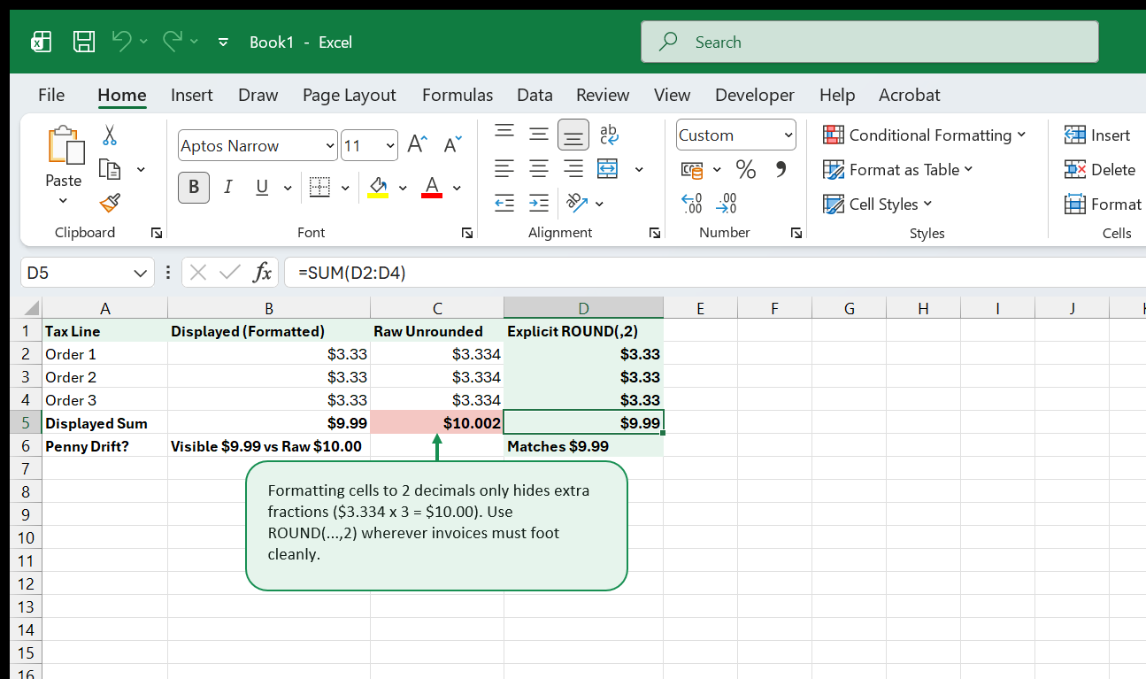
Even a workbook completely free of # error badges can fail a controller’s audit by $0.01 to $1.00. Why? Because formatting a cell as $#,##0.00 changes only the visual mask, never the underlying 15-digit IEEE floating-point value!
Look closely at three tax lines each holding 3.334:
- Formatted to
2decimals, Excel renders$3.33 + $3.33 + $3.33. - A human reading the printed PDF sums
3 × 3.33 = $9.99. - Unrounded
=SUM(C2:C4)computes3 × 3.334 = $10.002, which formats visibly as$10.00! Customers and auditors immediately reject invoices whose line items fail to foot to their printed total.
Chapter 11: Catching Circular References Before They Corrupt Cash Models
When a formula points directly or indirectly back to itself (B10 sums B2:B10 instead of B2:B9), Excel warns you once with a Circular References dialog, evaluates inconsistently or stalls at zero, and stamps “Circular References: B10” silently in the bottom-left status bar.
Finding Hidden Circular Chains Across Multi-Sheet Models
- Go to Formulas -> Error Checking dropdown -> Circular References.
- Notice the exact cell coordinates listed cleanly in that submenu (
Sheet3!E14). - Click the listed coordinate to jump straight onto the loop, then click Trace Precedents and Trace Dependents to spot which total row accidentally included itself—or where interest expense vs ending revolver debt created an intentional finance loop without Iterative Calculation enabled.
Chapter 12: Automated Sheet Reconciliation Checks
World-class models never trust luck after shipping. Reserve Rows 1–3 (or a dedicated Checks tab) for automated boolean control rows summed at the top-left corner of every tab (Master Check = "OK" / "ERROR"):
Standard 4-Check Reconciliation Block:
Check 1 (Balance Sheet Foot):    =ROUND(Assets - Liabilities_Equity, 2) = 0
Check 2 (Pivot vs Ledger Total): =ROUND(Summary!B20 - RawLedger!Z999, 2) = 0
Check 3 (Error Code Scan):       =COUNT(IF(ISERROR(Data!A1:Z500), 1)) = 0
Check 4 (Duplicate Key Scan):    =COUNTA(Data!A2:A500) = COUNTA(UNIQUE(Data!A2:A500))
Pair the top banner cell with bright red conditional formatting whenever Master Check <> "OK". The instant a single broken paste, missing lookup row, or rounding penny gap hits anywhere on a 20-tab workbook, your top header screams immediately before the PDF exports.
Chapter 13: The 5-Minute Workbook Rescue Protocol
Keep this fast emergency sequence bookmarked whenever someone hands you a broken file right before a meeting:
- Toggle
Ctrl + ~(Show Formulas): Check column consistency—confirm row 14 wasn’t overwritten with a typed manual override. - Press
F5 -> Special -> Formulas -> Errors: Highlight every single error cell across the whole active sheet in two seconds flat! - Trace Precedents (
Alt + M + P) on the earliest upstream broken cell: Never patch downstreamSUMKPIs until the origin error (#N/A,#DIV/0!, or text#VALUE!) clears cleanly. - Check Circular Reference status + Automatic Calculation mode (
Formulas -> Calculation Options -> Automatic): Verify someone did not leave the workbook stuck in Manual calculation mode showing stale numbers! - Run the Reconciliation Block check: Confirm row counts, grand totals, and
ROUND(..., 2)invoice totals match source exports to the final cent.
When you replace guesswork and blind IFERROR band-aids with structured auditing discipline, broken spreadsheets transform from stressful emergencies into two-minute routine diagnostics.
Chapter 14: Debugging Complex Nested Formulas With LET
Nested formulas spanning five lines (=IF(ISERROR(INDEX(..., MATCH(...))), 0, INDEX(..., MATCH(...)) * (1 - VLOOKUP(...)))) make even senior analysts lose track of which bracket closes which step.
Rewriting dense multi-step expressions with Microsoft 365 LET() cuts calculation work in half AND makes debugging transparent step by step:
=LET(
  cleanKey,   TRIM(SUBSTITUTE(A2, CHAR(160), " ")),
  rawPrice,   XLOOKUP(cleanKey, Master!$F$2:$F$100, Master!$G$2:$G$100, -1),
  validPrice, IF(rawPrice < 0, 0, rawPrice),
  validPrice * B2
)
Why does LET() supercharge auditing immediately? Because whenever an unexpected output shows up, you temporarily swap the final return expression from validPrice * B2 cleanly to cleanKey or rawPrice for three seconds to inspect exact intermediate outputs without dissecting 140 characters of nested parentheses!
Chapter 15: Troubleshooting Volatile Function Performance Drags
A workbook does not need #REF! errors to fail practically—if changing one assumption freezes Excel for 25 seconds showing “Calculating (8 Threads): 34%”, teammates turn calculation to Manual mode and accidentally publish stale numbers!
Watch out for Excel’s classic Volatile Functions (OFFSET, INDIRECT, TODAY, NOW, RAND, CELL, INFO), which recalculate 100% of dependent chains on every single keystroke anywhere in the workbook—even unrelated typing!
| Slow Volatile Pattern | Fast Non-Volatile Upgrade |
|---|---|
OFFSET(A1, 0, 0, COUNTA(A:A), 1) inside 2,000 rows |
Structured Excel Table column (tblData[Amount]) or INDEX(A:A, 1):INDEX(A:A, COUNTA(A:A)) |
INDIRECT("'Sheet" & A2 & "'!B5") across 500 links |
Consolidate regional sheets into one clean Table using SUMIFS / Power Query |
Entire-column array lookups (XLOOKUP(A2, Data!A:A, Data!B:B) legacy equivalents like SUMPRODUCT((A:A=x)*(B:B))) |
Bounded ranges or Excel Table references (Data!$A$2:$A$10000) |
Replacing 5,000 INDIRECT + OFFSET array cells cleanly with INDEX/XMATCH or Table refs routinely cuts recalculation latency from 18 seconds under 0.2 seconds cleanly.
Chapter 16: Locale, Date-System & Comma-vs-Semicolon Bugs
Ever email a flawlessly tested US workbook to a teammate in Germany, France, or Brazil—only to receive a screenshot filled with #VALUE! on imported date strings and broken CSV decimals?
Watch three silent cross-regional culprits:
- DMY vs MDY Date Strings (
"04/05/2026"): Excel text parsers read"04/05/2026"as April 5 on US machines and May 4 on UK/EU machines—or reject"05/18/2026"completely as non-date plain text (#VALUE!) in London! Always construct dates viaDATE(2026, 4, 5)or ISO"2026-04-05", never locale-dependent slashed strings inside formulas. - Formula Separators & Decimal Formats: Excel translates core function names automatically on open (
SUM->SOMMEin French), yet inline text strings passed intoNUMBERVALUE(A2, ".", ",")OR hardcodedTEXT(B2, "yyyy-mm-dd")format masks may vary when date mask tokens change across locales. Test European decimal strings cleanly with explicitNUMBERVALUE(str, decimal_sep, group_sep). - 1900 vs 1904 Date System Drift (
+1462Days): Pasting dates between legacy Mac 1904-epoch workbooks and Windows 1900-epoch files silently shifts every date by 4 years and 1 day! Always verify File -> Options -> Advanced -> When calculating this workbook -> Use 1904 date system stays UNCHECKED consistently.
Chapter 17: Inspecting Workbook Bloat, Ghost Styles & Phantom UsedRanges
Sometimes a tiny 500-row spreadsheet balloons to 28 MB, takes 40 seconds to save, or spawns vertical scrollbars jumping straight to row 1,048,576.
Diagnose and cure structural corruption fast:
- Fix Phantom Scrollbars (
UsedRangebloat): PressCtrl + Endon every worksheet. If the cursor jumps onto empty CellXFD1048576instead of the bottom-right corner of your real table, highlight all empty rows below your last real row -> Home -> Clear -> Clear All (or delete whole rows cleanly), repeat for empty columns right of data, and Save (Ctrl + S) immediately so Excel resetsUsedRange. - Inspect Hidden
VeryHiddenTabs & Phantom External Links: Open Data -> Queries & Connections -> Edit Links (Workbook Links) cleanly to spot deadC:\Users\OldAnalyst\Budget.xlsxlinks triggering slow open prompts, and check Home -> Find & Select -> Selection Pane for invisible stray shapes left stacked over cells.
Chapter 18: Interactive Error-Hunt Lab (6 Classic Traps Diagnosed Live)
Test your diagnostic reflexes against six real field scenarios encountered during monthly closes:
| Case | Symptom Observed | Exact Root Cause Discovered | Fast Fix Applied |
|---|---|---|---|
| Case 1 | =SUM(B2:B50) shows 0 despite visible numbers |
ERP export padded leading apostrophes / spaces turning column to text | Text-to-Columns Finish OR =SUM(NUMBERVALUE(...)) |
| Case 2 | =VLOOKUP("204", A:C, 3, FALSE) returns #N/A on visible 204 |
Lookup argument "204" is text; Table column stores integer 204 |
Match types (=XLOOKUP(--A2, ...)) |
| Case 3 | Updating cell D4 turns whole column to 0 (Circular Ref) |
Row D12 Total accidentally summed =SUM(D2:D12) including itself |
Fix range strictly to =SUM(D2:D11) |
| Case 4 | Adding 1 row to B20 silently skipped from summary KPI |
Hardcoded =SUM(B2:B19) missed appended rows below range |
Convert source range to Ctrl+T Table cleanly |
| Case 5 | #SPILL! inside an Excel Table after pasting UNIQUE() |
Formatted Ctrl+T Tables forbid multi-cell dynamic spill arrays |
Place UNIQUE() dashboard summaries outside Table boundaries |
| Case 6 | Balance Sheet off by $0.01 on printed invoice PDF |
Cell visual formatting masked $3.334 underlying decimal fractions |
Wrap invoice line tax math in =ROUND(..., 2) |
Chapter 19: Building Self-Healing Audit Dashboards
Top spreadsheet engineers embed debugging directly into every production template rather than running frantic fire drills every month-end:
- Create a top-row
AUDIT_STATUSRibbon on Tab 1: Aggregate four boolean gates across all worksheets cleanly (=IF(AND(FootOK, NoErrorCells, UniqueKeysOK, LinkHealthOK), "ALL CHECKS PASS", "REVIEW REQUIRED")). - Count Formula Errors Silently Across Sheets (
ISERROR): Run clean helper counters targeting critical columns (=SUMPRODUCT(--ISERROR(Ledger!F2:F2000))) so a single#VALUE!or#N/Ahiding on Row1,488alarms Tab 1 immediately in bright crimson! - Never Ship With Stale Calculation Modes: Make checking Formulas -> Calculation Options = Automatic the very final step of your signoff ritual before sending
.xlsxor PDF deliverables cleanly to leadership.
That's the whole book. Keep the PDF for offline reading.
Downloading requires a free Google sign-in -- reading online never does.