
This book is about the Power Query workflow itself - the editor, the steps, the habits - not a general guide to cleaning data. If you’re still deciding whether your data needs Power Query at all, or you’re doing the prep work on the Excel side before a report connects to it, preparing Excel data for a clean handoff covers that angle instead; this book picks up once you’ve decided to actually use Power Query.
What Power Query Is (and Why It Beats Manual Cleanup)
Power Query is Excel’s built-in tool for pulling in data and reshaping it - from a table already in your workbook, a CSV file, a database, or a web page - through a sequence of named, ordered steps that stay attached to the result. Change the source data, click Refresh, and every step reruns automatically, in order, against the new data.
That last sentence is the entire reason to use it. Manually cleaning a spreadsheet - deleting a column, filtering out some rows, fixing a data type - produces a clean result once. The moment a new export of the same report arrives, all of that work has to be redone from scratch, by hand, identically, forever. Power Query records what you did as a reusable recipe instead of a one-time action: the same filter, the same split, the same de-duplication, reapplied automatically every time the source changes.
That tradeoff has a real cost, though - a query takes a few minutes longer to set up the first time than just fixing the data directly would. For a one-off file you’ll genuinely never touch again, that setup time doesn’t pay for itself; the CSV cleaner tool on this site does trim/dedupe/blank-row-removal instantly for exactly that case. Reach for Power Query once you’re repeating the same cleanup on a recurring report - weekly sales exports, a monthly reconciliation, anything you’d otherwise redo by hand next month.
Importing Data
Every Power Query starts the same way: Data → Get Data, then a choice of source. Two are worth knowing cold before anything else.
From a Table or Range
The easiest way in, and the one to practice on first: click inside any data already in your workbook, then Data → Get Data → From Table/Range (or From Sheet, depending on your Excel version - same feature).
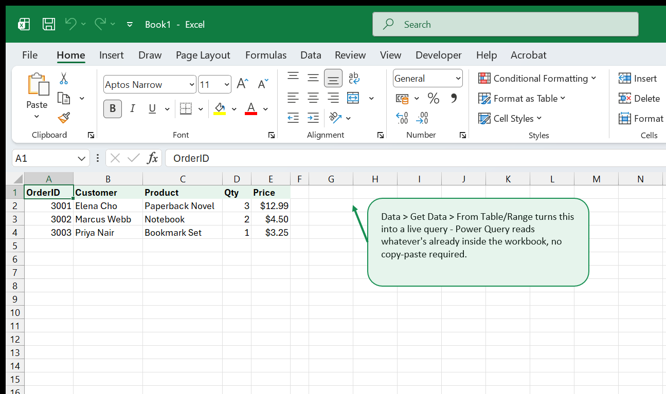
If the range isn’t already a formatted Excel Table, Excel offers to convert it into one first (it needs a defined, named boundary to query against). This opens the Power Query Editor - a separate window with your data shown in a grid and an Applied Steps list down the right side. That list is the whole point of Power Query: every transform you make from here on gets recorded as a named step, in order, and can be edited, reordered, or removed later without starting over.
From a CSV File
Data → Get Data → From Text/CSV, then pick a file. The same Power Query Editor opens, showing a preview of the file’s contents before you commit to loading anything - useful for catching an obviously wrong delimiter or encoding before it becomes fifty rows of garbled text in your workbook.
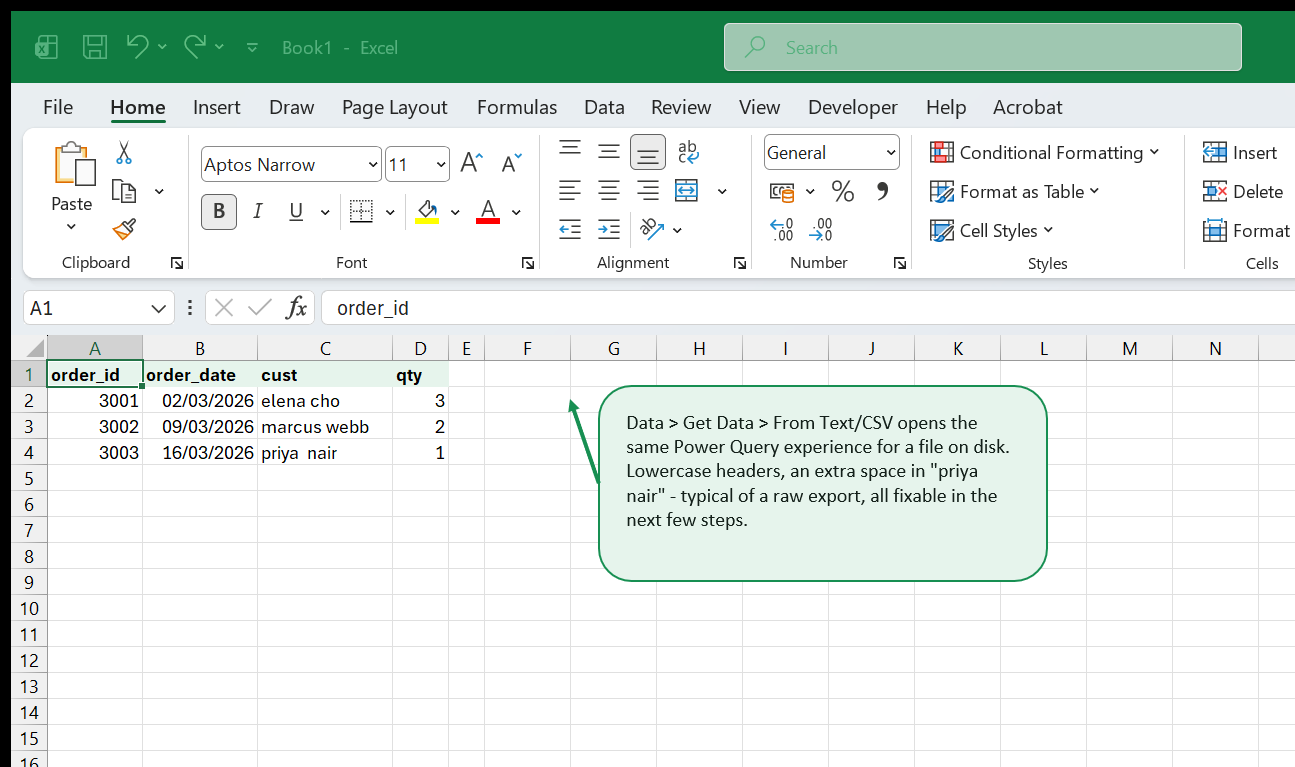
CSV exports are frequently the messiest source you’ll import: inconsistent header casing, stray whitespace, numbers and dates stored as plain text with no type information at all (a CSV file has no concept of a “date column” - everything in it is text until something tells Excel otherwise). Every core transform in the next chapter addresses exactly one piece of that mess.
The Core Transforms
Five operations cover the large majority of real cleanup work. Each one becomes its own line in the Applied Steps list - editable, reorderable, or deletable later without redoing anything that came before or after it.
Remove Columns
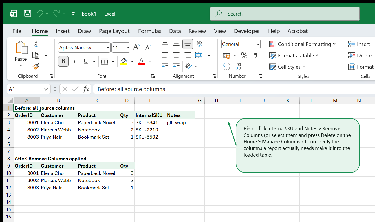
Right-click any column header in the Power Query Editor and choose Remove, or select several and use Home → Remove Columns. Only the columns a report actually needs make it into the loaded table - an internal SKU code or a free-text notes field that nobody downstream reads doesn’t need to travel any further than the source file.
Filter Rows
The dropdown arrow on any column header in the editor works exactly like a worksheet AutoFilter - untick values to exclude, or use the text/number filter submenus for “contains,” “greater than,” “between,” and similar conditions. Unlike a worksheet filter, this doesn’t just hide rows - it genuinely removes them from the query’s result, and the removal reruns automatically on refresh, matching whatever rows meet the condition in the new data.
Change Data Types
Click the small type icon in a column header (ABC for text, 12 for whole numbers, a calendar for dates, and so on) and choose the correct type, or select Change Type for more options. This matters more than it looks like it should: a date stored as text sorts alphabetically instead of chronologically, and a number stored as text can’t be summed, averaged, or compared correctly by anything downstream.
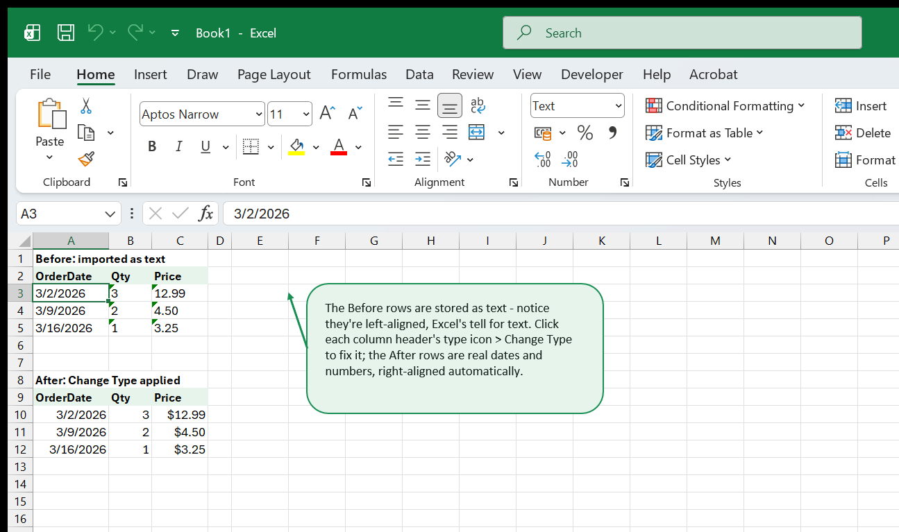
The tell shown here - left-aligned “Before” values, right-aligned “After” ones - works the same way directly on a worksheet, not just inside Power Query: if a column of numbers looks stubbornly left-justified, that’s Excel telling you it’s text, before you even open Format Cells to check.
Split a Column
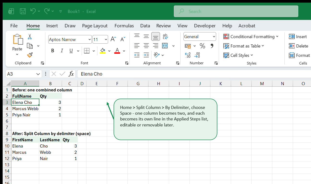
Home → Split Column → By Delimiter breaks one column into several wherever a chosen character appears - a space, a comma, a hyphen. A single “Full Name” column becomes separate First Name and Last Name columns in one step, no formula written by hand.
Remove Duplicates
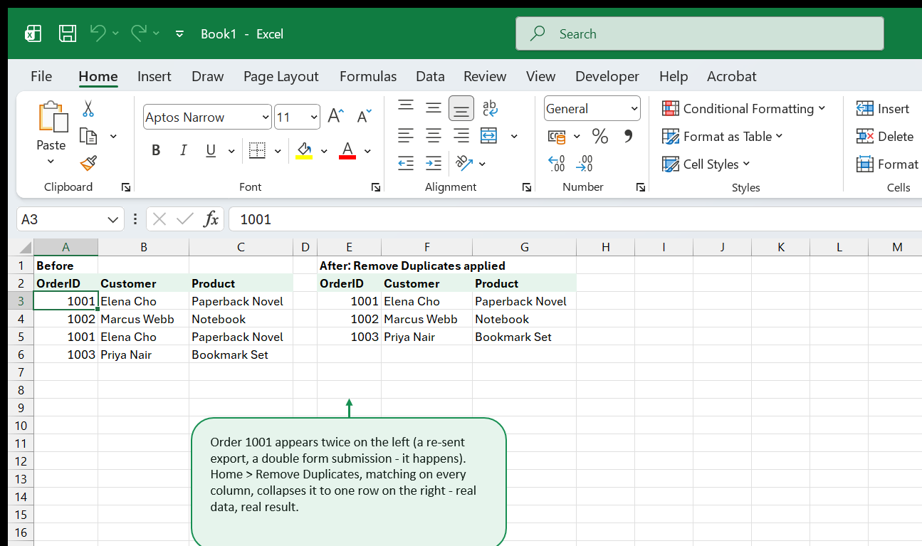
Select the relevant column(s) - or the whole table for an exact full-row match - and use Home → Remove Duplicates. The first occurrence of each unique combination is kept; every later repeat is dropped.
Reach for messy data cleanup practice - a dataset built specifically with extra whitespace, mixed case, duplicate rows, and numbers stored as text - to try all five of these transforms together on one file.
Combining Two Queries: Append
Two recurring exports with the same columns but different rows - an online store’s orders and an in-store POS system’s orders, say - need stacking on top of each other, not merging side by side. That’s Home → Append Queries: pick a second query, and its rows get added underneath the first query’s rows into one combined result.
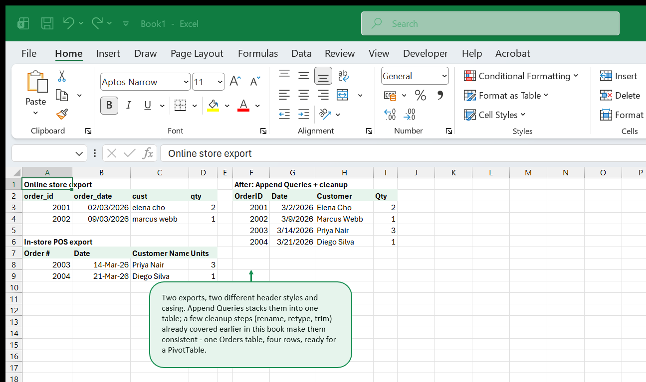
Append rarely works well as the very first step - two real-world exports
almost never share identical column names or casing straight out of the
box, the way the two sources above didn’t (order_id/cust vs. Order #/Customer Name). The practical order is almost always: clean up each
source query on its own first (rename columns to match, fix data types,
trim stray whitespace) so both queries expose the exact same column names
in the exact same order, then append them. Skipping that step doesn’t
throw an error - it just produces a combined table with extra, oddly
mismatched columns instead of one clean one, which is a confusing thing to
debug after the fact.
Merge Queries is a different, related command worth knowing exists, even though this book doesn’t cover it in depth: instead of stacking rows, it joins two queries side by side on a matching column - the same idea as a lookup formula, but query-to-query instead of value-to-value.
Refresh Behavior
The entire reason to use Power Query instead of a one-time manual cleanup: right-click the loaded table (or any cell in it) and choose Refresh, or Data → Refresh All to refresh every query, connection, and PivotTable in the workbook at once. Every recorded step - the column removal, the filter, the type change, the split, the de-duplication, the append - reruns automatically against whatever the source looks like now.
A few things worth knowing about what refresh does and doesn’t do:
- It reruns the steps, not the original result. If the source CSV gains a new column, a query that explicitly removed columns by name simply ignores the new one (nothing to remove); a step that instead kept a fixed list of columns to retain would drop it automatically. Which behavior you get depends on exactly how the step was built - worth a quick check in Applied Steps after a source file’s shape changes.
- A query can be set to refresh automatically when the file opens - right-click the query in the Queries & Connections pane → Properties → “Refresh data when opening the file.” Off by default.
- Refreshing a query is separate from refreshing a PivotTable built on top of it - a pivot has its own, similarly named “Refresh data when opening the file” option under its own PivotTable Options. Building a small report that chains a CSV import → a query → a PivotTable means checking both settings if you want the whole chain to update itself on open.
- A broken source (a renamed file, a moved folder) doesn’t fail silently - refresh throws a visible error naming the query that couldn’t run, rather than quietly serving stale data.
Common Pitfalls
- Appending before cleaning up column names. Covered above - clean each source query to matching column names and types first, or Append produces a confusing, oddly-columned result instead of an error.
- A CSV column imported as text staying that way silently. Nothing visually dramatic happens - the column just won’t sum, sort chronologically, or filter numerically correctly until Change Type is applied. Check alignment (left = text, right = number/date) as a quick visual tell, on a worksheet or inside the query editor alike.
- Removing rows/columns from the loaded table instead of the query. Deleting a row directly in the worksheet only removes it until the next refresh brings it right back - the fix belongs in a Filter Rows step inside the query, not as a manual edit downstream of it.
- Forgetting that Refresh and “refresh on open” are two different settings - covered above, and the second one is off by default even after you’ve refreshed manually once.
- Treating Power Query as a one-time cleanup tool. It can be used that way, but the entire value case is recurring, refreshable cleanup - a single-use file is usually faster to fix directly, as the first chapter covers.
Quick Reference
| Task | How |
|---|---|
| Start a query from data already in the workbook | Data → Get Data → From Table/Range |
| Start a query from a CSV file | Data → Get Data → From Text/CSV |
| Remove a column | Right-click its header → Remove, or Home → Remove Columns |
| Filter which rows stay | The dropdown arrow on any column header |
| Fix a column’s data type | Click the type icon in the column header, or Transform → Data Type |
| Split one column into several | Home → Split Column → By Delimiter |
| Drop duplicate rows | Select columns → Home → Remove Duplicates |
| Stack two queries’ rows together | Home → Append Queries |
| Join two queries side by side | Home → Merge Queries |
| Send the finished result to a worksheet | Home → Close & Load |
| Rerun every step against updated source data | Right-click the table → Refresh, or Data → Refresh All |
| Auto-refresh when the file opens | Queries & Connections pane → query Properties |
Where to Go Next
- Getting started with Power Query is a shorter companion covering the same first steps from a different angle.
- Power Query refresh checklist goes deeper on the refresh-behavior chapter above - worth reading before building anything you plan to reuse regularly.
- Power Query vs. Excel formulas and Power Query vs. VBA for data cleanup cover when each tool is the better choice for a given cleanup job.
- Preparing Excel data for a clean Power BI handoff picks up right where this book leaves off if a Power BI report is the next destination - the same query steps carry over almost unchanged, since Power Query is the identical engine underneath both tools.
- Browse the Power Query topic for more articles beyond this book.
- Practice on messy data cleanup practice - built specifically for the five core transforms covered here.
- Once your cleaned data needs summarizing rather than just cleaning, Pivot Tables from Zero is the natural next step - a Power Query result loads straight into a PivotTable the same way any other Excel Table does.
- New to Excel entirely? Excel for Beginners covers the fundamentals this book assumes you already have.
That's the whole book. Keep the PDF for offline reading.
Downloading requires a free Google sign-in -- reading online never does.