
Most Excel users learn how to drop one field into Rows and one field into Values, nod at the subtotal table, and stop there. That gets you across the first bridge — summarizing a clean flat table in thirty seconds — and it is exactly what Pivot Tables from Zero teaches well.
Volume 2 picks up where basic one-column PivotTables run out of headroom. Real reporting asks harder questions: how did each tool and paint category perform inside every sales region, how do Q1 and Q2 sit side by side across channels, what share of total revenue does each line represent, and how can a non-technical manager filter the entire report with two clicks instead of digging through hidden header menus?
Throughout all twelve chapters we use a unified hardware-supply wholesale ledger (Northside Tool & Supply, tracking transactions across North, South, and West warehouses, Tools, Paint, and Safety categories, Online vs. Retail channels, and quarterly order volumes). Every PivotTable layout, formula calculation, and slicer design in this volume comes straight from a live Excel workbook so you can reproduce every view step by step.
1. Flat-Table Discipline for Multi-Pivot Workbooks
Goal: Design a clean transactional table that never breaks multi-level PivotTables, calculated percentages, or slicers when new months are appended.
Before dragging a single field into a PivotTable Field List, look critically at your source sheet. Most PivotTable frustrations — broken date grouping, (blank) subtotal rows, text columns that refuse to sort numerically, or "Count of Revenue" instead of "Sum of Revenue" — trace back to structural shortcuts in the source grid rather than the Pivot engine itself.
Converting Raw Extracts into Official Tables
Always store your source dataset inside an official Excel Table (Ctrl + T, named cleanly under Table Design → Table Name, such as tblOrders). An Excel Table gives every downstream PivotTable three structural guarantees:
- Elastic Boundaries: Appending row 501 automatically stretches the Table range. Clicking Data → Refresh All absorbs new sales with zero
Change Data Sourceedits. - Typed Columns: Every column header is unique and non-blank, avoiding cryptic
Column1fields inside the Pivot Field List. - Zero Subtotal Pollution: Totals belong in a Total Row (
Table Design → Total Row) or in the PivotTable itself — never inside rows of source transactions. Mixing summary rows into raw data doubles your grand totals instantly.
Why Blank Cells Flip Sum to Count
Even one empty cell or stray text note inside a numeric Revenue column forces Excel’s Pivot engine to switch the default aggregation to Count. Before inserting a PivotTable, select the data body of any numeric column and glance at the Status Bar: if both Count and Sum appear, every cell is numeric; if only Count appears, non-numeric entries are hiding inside that range.
| Structural Check | Broken Source Symptom | Volume 2 Standard |
|---|---|---|
| Merged header rows | Pivot Field List refuses to build | Single flat header row (A1:G1) |
| Cross-tab month columns | Must drag 12 separate Jan–Dec fields | One Date or Quarter column (Power Query Unpivot) |
| Embedded subtotals | Grand Totals double-count records | Keep transaction rows purely granular |
Blank cells in Units |
Summarizes by Count instead of Sum | Populate explicit zeros (0) cleanly |
2. Multi-Level Row Hierarchies & Collapsible Outlines
Goal: Nest multiple categorical fields inside the Rows area to drill cleanly from regional performance down to product-line subtotals.
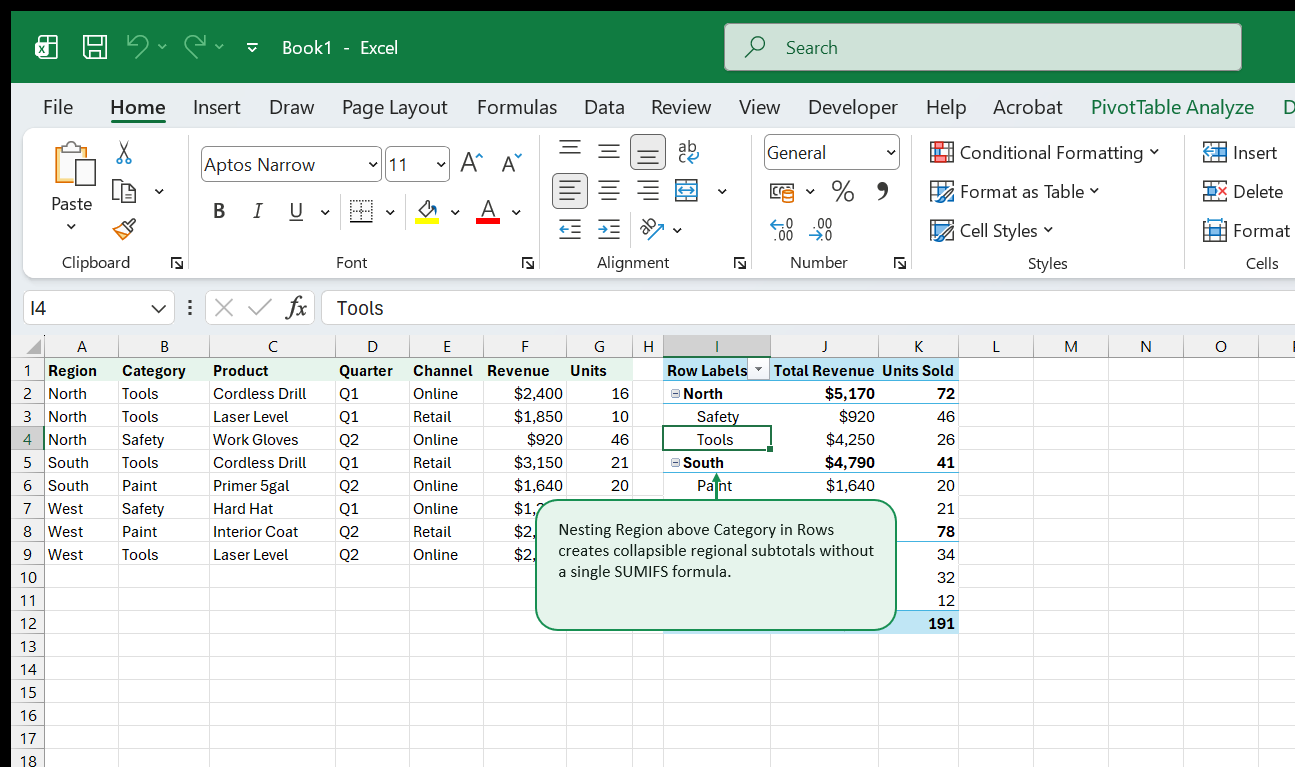
A flat category summary hides regional problems. Total Tools sales might look healthy globally while North warehouse tool sales collapse. Nesting two or three fields vertically inside the Rows area solves this without writing a single nested SUMIFS formula.
Nesting Order Determines the Story
Dragging Region first and Category directly underneath it inside Rows produces an indented hierarchy where every region acts as a collapsible parent folder containing its own product categories. Reversing the order (Category above Region) pivots the entire narrative from warehouse management to category performance across warehouses.
Choosing Report Layouts That Export Cleanly
By default, Excel builds multi-row PivotTables in Compact Form, squeezing both Region and Category into Column A. While compact on screen, copying Compact Form downstream into formulas breaks cleanly aligned columns. Instead, open Design → Report Layout and keep two deliberate alternatives ready:
- Outline Form: Pushes each nested field into its own column while preserving expandable parent rows and top subtotals. Ideal for interactive review meetings.
- Tabular Form + Repeat All Item Labels: Places every field in its own clean column and repeats parent region names on every line (
Design → Report Layout → Repeat All Item Labels). Whenever you plan to feed Pivot output into downstream charts or export to CSV, Tabular Form eliminates blank left cells cleanly.
Expanding and Collapsing Whole Levels at Once
Instead of clicking dozens of tiny [+] / [-] buttons individually, right-click any outer region label (North, South, or West) and choose Expand/Collapse → Collapse Entire Field for an instant three-row regional executive summary, or Expand Entire Field to audit category detail across every branch simultaneously.
3. Cross-Tab Matrices with Columns & Multi-Value Headers
Goal: Build two-dimensional quarterly comparison matrices using both the Rows and Columns drop zones cleanly.
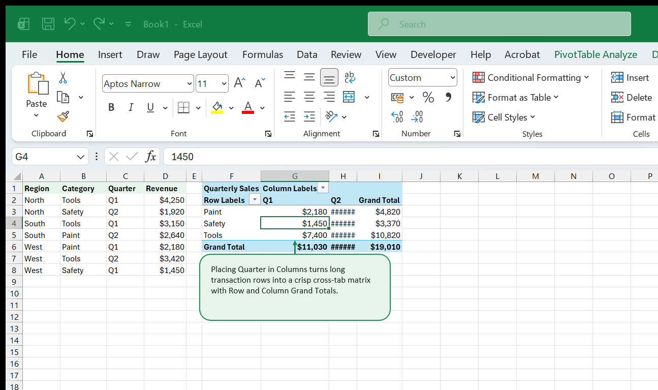
Vertical lists excel at drilling deep into hierarchy; two-dimensional matrices excel at spotting time trends or channel shifts across categories. Moving a discrete grouping field such as Quarter or Channel into the Columns zone stretches categories horizontally so readers can scan Q1 vs. Q2 side by side in a fraction of a second.
Managing the “Values” Pill Automatically
Notice what happens inside the Field List the moment you add two numeric fields (such as Total Revenue and Units Sold) alongside a Column field: Excel spawns a synthetic Σ Values pill inside either Columns or Rows. Dragging Σ Values below Quarter groups Q1 Revenue | Q1 Units next to Q2 Revenue | Q2 Units. Dragging Σ Values into Rows stacks Revenue and Units as clean alternating rows beneath each category, often saving horizontal width on narrow screens and PDF printouts.
Controlling Grand Totals & Subtotals Intentionally
Not every matrix needs four edges of totals. When comparing Average Margin % or Unit Price across quarters, summing percentages across columns produces nonsense numbers. Under Design → Grand Totals, select On for Rows Only or Off for Rows and Columns selectively so managers never mistake a summed rate for a meaningful metric.
4. Customizing Value Aggregation & Number Formats Permanently
Goal: Rename cryptic “Sum of Revenue” headers cleanly and lock currency formatting so refreshes never strip styling.
Fresh PivotTables default to clunky headers like Sum of Revenue and Count of Product formatted in plain unformatted General digits. Formatting the cells using the Home tab Number Format toolbar is one of the most common mistakes in Excel: the moment new rows arrive and the Pivot shrinks or grows on refresh, direct cell formats lag behind or wipe cleanly off new rows.
Format Through Value Field Settings Instead
Always double-click the numeric column header inside the PivotTable (or click Value Field Settings… in the Values drop zone) and click the bottom-left Number Format button inside the dialog box. Applying $#,##0 there binds formatting to the field metadata itself rather than coordinates on the sheet grid, guaranteeing crisp dollar signs no matter how filters shift the table height.
Giving Clean Custom Names Without Colliding
Excel refuses to let you rename Sum of Revenue to bare Revenue because that exact string already exists as a source column name in your raw table. Solve that cleanly in two ways:
- Use a crisp descriptive phrase like
Total RevenueorQuarterly Sales. - Or append a single trailing space (
"Revenue ") when compact single-word headers matter visually.
Mixing Sum, Count, Average, Min, and Max Side by Side
You can drag the exact same numeric field (Revenue) into Values twice — once summarized by Sum (Total Revenue) and a second time summarized by Average (Avg Order Size) or Count (Order Count). Paired together, executives can verify whether a spike in North revenue came from heavier order volume or larger individual order sizes.
5. Show Values As: Mix Percentages, Running Totals & Period Variances
Goal: Turn raw summed dollars into % of Grand Total, % of Parent Row, running totals, and period-over-period growth inside native Pivot Settings.
Adding helper formula columns next to a PivotTable is fragile: if a slicer narrows the PivotTable from 12 rows down to 4 rows, external formulas beside rows 5 through 12 dangle in mid-air returning #REF! or stale 0% artifacts. Native Show Values As calculations sit inside the Pivot cache and resize seamlessly alongside every slice.

Five High-Impact Show Values As Modes
Right-click any number inside a Pivot Value column and explore Show Values As:
| Mode | Question Answered | Practical Example |
|---|---|---|
% of Grand Total |
What share of overall business is each slice? | Tools drives 51.5% of total revenue |
% of Column Total |
Within Q2, which region carried volume? | Comparing regional mix shifts quarter to quarter |
% of Parent Row Total |
Inside North warehouse, what is Paint’s mix? | Multi-level audit keeping each branch summing to 100% |
Difference From (Previous) |
Did sales grow vs. prior period in dollars? | Q2 variance minus Q1 baseline (+$1,420) |
Running Total In |
What is cumulative YTD performance? | Cumulative revenue tracking through Dec |
Pairing a raw dollar column alongside a duplicated % of Grand Total column inside the exact same PivotTable delivers executive-ready mix insights without leaving the Field List.
6. Visual Filtering with Slicers & Connected Report Grids
Goal: Replace cramped header dropdown arrows with tactile, color-coded Slicers connected across multiple PivotTables and charts simultaneously.
Hidden AutoFilter dropdown arrows inside Pivot row headers are terrible for shared workbooks: readers cannot tell at a glance which regions are active, and clicking through checkboxes to test two combinations takes half a dozen clicks per view. Slicers transform filters into visible, self-documenting dashboard controls.

Formatting Slicers Like Real App Controls
Click inside a Slicer to unlock the Slicer contextual tab:
- Increase Columns from
1to2or3inside horizontal top filter bars so three regions fit inside a sleek horizontal ribbon instead of consuming vertical spreadsheet height. - Enable Slicer Settings → Hide items with no data so stale seasonal codes sink cleanly to the bottom grayed out (or vanish altogether).
- Right-click any Slicer and choose Report Connections… to wire one
Regionslicer to three separate PivotTables and two PivotCharts on a dashboard sheet at once. Clicking West updates every tile, chart, and summary simultaneously.
7. Report Filter Pages & Top-Level Scoping
Goal: Scope an entire summary cleanly using the Filters drop zone, and split one PivotTemplate into thirty regional sheets in two seconds with Show Report Filter Pages.
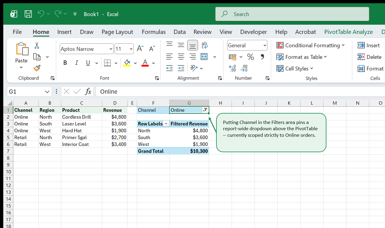
Not every filter belongs as a flashy button on screen. Placing Channel into the Filters zone pins a compact selector cleanly above Row 1 — ideal when setting a global report view (such as isolating strictly Online orders before printing a channel packet).
One-Click Workbook Tab Multiplication
One of Excel’s best hidden productivity shortcuts sits inside PivotTable Analyze → Options (dropdown arrow) → Show Report Filter Pages…: whenever a PivotTable has a field in the Filters box (Region, Department, or SalesRep), clicking Show Report Filter Pages clones the entire formatted PivotTable onto dedicated tabs — one worksheet per unique value (North, South, West), each pre-filtered cleanly for packet distribution or PDF export!
8. Dynamic Sorting, Ranking & Top-10 Value Filters
Goal: Sort products strictly by revenue volume (not A–Z alphabet) and restrict busy PivotTables to Top-N performers dynamically.
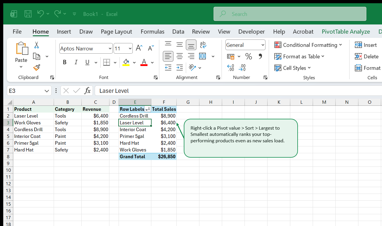
By default, every Excel PivotTable sorts Row labels alphabetically (Cordless Drill, Hard Hat, Interior Coat…). Alphabetical sorting tells managers zero about what drives revenue. Always sort your core business breakdowns descending by numeric metric instead.
Applying Dynamic Top-10 Filters
When your catalog holds 400 SKUs, showing every Work Gloves tail SKU drowns out key movers. Click the Row Header filter arrow → Value Filters → Top 10… and filter Products by Top 5 Items by Total Sales. Crucially, remember to sort descending alongside Top 5 filtering — Top 5 narrows which items remain, while descending Sort orders those 5 champions cleanly from #1 down to #5.
9. Calculated Fields vs. Power Query Pre-Calculations
Goal: Understand when lightweight Pivot Calculated Fields work smoothly, when weighted-average math breaks them, and when to compute columns upstream instead.
Suppose your source ledger stores Qty and Price separately, or Revenue and Margin Dollars. You want Gross Margin % right inside the PivotTable. Under PivotTable Analyze → Fields, Items, & Sets → Calculated Field, typing = Margin / Revenue yields a true weighted ratio across every Pivot subtotal (Sum(Margin) / Sum(Revenue)), which simply averaging a source Margin% column would get dead wrong!
When Calculated Fields Break Down
Be wary of two classic Calculated Field traps:
- Multiplying at row vs. aggregate level: A Calculated Field literally applies
= SUM(Qty) * SUM(Price)at subtotal levels! Multiplying quantities by prices must happen row-by-row inside your Excel Table (=[@Qty]*[@Price]) or Power Query before loading into the Pivot cache. - Zero-denominator
#DIV/0!cells: Wrap ratio fields safely as= IF(Revenue=0, 0, Margin/Revenue)or move complex multi-table ratios into Power Pivot DAX (DIVIDE) covered in our Power Pivot & DAX Field Guide.
10. Custom GETPIVOTDATA Extraction for Polished Reports
Goal: Build pixel-perfect executive report layouts fed dynamically from live PivotTables using GETPIVOTDATA without worrying about shifting row numbers.
Typing =B14 to reference a Pivot subtotal on a formatted cover sheet feels fast until a filter collapses B14 into a Grand Total row or removes it completely. Instead, clicking any cell inside a PivotTable while typing a formula triggers Excel’s built-in GETPIVOTDATA:
=GETPIVOTDATA("Revenue", $F$1, "Region", "North", "Category", "Tools", "Channel", "Online")By replacing hard-coded string literals ("North") with cell references ($A$3), one clean structured report grid pulls live Pivot aggregates even when rows expand, collapse, or resort alphabetically underneath! Want ordinary relative drag-formulas (=F4+G4) instead? Uncheck PivotTable Analyze → Options → Generate GetPivotData temporarily, or type coordinates directly.
11. PivotCharts & Interactive Executive Views
Goal: Link live PivotCharts smoothly while stripping noisy Field Buttons and preserving color discipline across slicer updates.
Clicking PivotTable Analyze → PivotChart drops an interactive chart wired straight to your Pivot cache: slicing Region updates both table and chart immediately. Yet default PivotCharts arrive cluttered with gray Field Buttons overlapping plot edges and generic legends.
Five-Step PivotChart Polish Checklist
- Right-click any gray Field Button on the chart → Hide All Field Buttons on Chart.
- Set
Chart Design → Add Chart Element → Legend → ToporBottom(never right margin squishing columns). - Sort the underlying PivotTable descending so horizontal bars cascade neatly longest-to-shortest like our Excel Charts & Data Visualization standards.
- Keep Autofit column widths on update unchecked in PivotTable Options (
Layout & Formattab) when positioning charts cleanly adjacent to tables so refreshing long category text never squishes your dashboard grid! - Save recurring layouts safely by backing up clean source patterns on ExcelBack Templates and practicing on real multi-sheet files via ExcelBack Datasets.
12. Performance, Caching & Where to Go Next
Goal: Keep large multi-Pivot workbooks fast, prevent stale cache bloat, and choose your next specialization smoothly.
Whenever you copy-paste an existing PivotTable (Ctrl+C / Ctrl+V), both tables share one underlying memory cache — clicking Refresh once updates both together and keeps file sizes small. Beware, however, when two Pivots share a cache: grouping Dates by Month in one forces Month grouping across every companion Pivot wired to that same cache!
Refresh Habits That Prevent Stale Numbers
- Right-click → PivotTable Options → Data tab → Refresh data when opening the file ensures Monday morning stakeholders never read Friday’s numbers.
- Set Number of items to retain per field to None (Data tab) so deleted discontinued SKUs vanish permanently from Slicer lists upon refresh instead of lingering as ghost buttons.
Continue Your Learning on ExcelBack
- Automate messy source prep before Pivots: Power Query & M Transformations (Volume 2) shows how Unpivot turns wide monthly spreadsheets into clean Pivot-ready tables automatically.
- Unlock DAX Measures & Multi-Table Stars: Power Pivot & DAX Field Guide takes you past single flat-table Pivot limits into relational sales models.
- Test individual functions interactively: Browse Excel Functions Reference or clean an export immediately using our browser CSV Cleaner Tool.
13. Date Grouping Mysteries & Custom Fiscal Hierarchies
Goal: Control Excel’s automatic date grouping behavior so fiscal years, ISO weeks, and custom 4-4-5 calendars aggregate cleanly instead of scattering months into alphabetical order.
The moment you drag a Date column into PivotTable Rows or Columns, Excel automatically creates three hidden virtual fields (Years, Quarters, Months). While handy for calendar-year reporting, automatic grouping breaks down in three common situations:
- One non-date cell in the source column: A single
"TBD", trailing space, or blank string disables Pivot date grouping for all50,000rows simultaneously (Cannot group that selection). - Non-January Fiscal Years (e.g., April 1 or July 1 starts): Native PivotTable grouping hardcodes
Q1 = Jan–Marand cannot shift fiscal quarters to July starts cleanly. - Separate Pivots sharing a cache: Grouping months on Pivot A silently alters ungrouped raw dates on Pivot B if both Pivots share the same underlying PivotCache!
Explicit Calendar Columns Beat Auto-Grouping
For durable Northside Tool & Supply reporting, generate explicit calendar columns right inside your source tblOrders table (FiscalYear, FiscalQuarter, MonthSort, YearMonthLabel):
="FY"&(YEAR(A2)+IF(MONTH(A2)>=7,1,0))&"-Q"&ROUNDUP(MOD(MONTH(A2)-7,12)/3+0.1,0)Even better: build a clean Fiscal Calendar Dimension Table and join it in the Excel Data Model so sorting MonthName by MonthNumber keeps Jul, Aug, Sep ... Jun in exact chronological sequence across every workbook tab.
14. Dynamic Date Windows & Grouping by Numeric Buckets
Goal: Segment wholesale invoice totals by order size tier (<$1K, $1K–$5K, $5K+) and summarize 7-day rolling weekly order buckets cleanly without helper formulas.
Beyond date hierarchies, right-clicking any numeric row field (for instance, OrderAmount in Rows) and clicking Group… opens Excel’s numeric binning dialog (Starting at: 0, Ending at: 10000, By: 1000). Within five seconds, raw order amounts group into readable deal-size bands:
| Deal Size Bucket | Pivot Row Output | Orders | Total Revenue | Avg Order |
|---|---|---|---|---|
0–999 |
Micro Restock | 184 | $98,400 | $535 |
1,000–2,999 |
Mid-Market Order | 112 | $214,800 | $1,918 |
3,000–4,999 |
Regional Restock | 49 | $188,650 | $3,850 |
>= 5,000 |
National Fleet Deal | 19 | $162,400 | $8,547 |
Grouping Days into Rolling 7-Day Sprints
To compare exact 7-day or 14-day promotional sprints instead of variable 28/30/31-day calendar months:
- Ungroup automatic
Years / Quarters / Months(Right-click -> Ungroup). - Open Group…, select Days only (deselect Months and Quarters!), set Number of days = 7, and anchor Starting at onto your campaign Monday (
2026-01-05).
Because PivotTable caches align Monday-to-Sunday weeks uniformly, Retail vs Online launch comparisons stop suffering from 4-weekend vs 5-weekend calendar distortions.
15. Calculated Fields vs Calculated Items: When Each Fails
Goal: Understand the silent traps inside PivotTable Calculated Fields (wrong weighted averages and subtotals) versus Power Pivot DAX measures.
Built-in PivotTable Fields, Items, & Sets -> Calculated Field looks convenient for margins: you write = Margin / Revenue, click Add, and get a clean Margin % column. Yet Calculated Fields follow one rigid algebraic rule: Excel sums each numerator and denominator FIRST, then evaluates your formula—even on subtotals and custom unit prices!
- Where Calculated Fields Work: Weighted ratios such as
Total Margin % = SUM(Profit) / SUM(Revenue)aggregate correctly at every subtotal level (North,South,Grand Total). - Where Calculated Fields Lie Silently: Multiplying
Quantity * UnitPrice(= Units * Price) inside a Calculated Field adds all Units (400) and sums all Unit Prices (\$1,250) first, reporting400 * \$1,250 = \$500,000instead of true row-by-row extended revenue! Always compute row-level products inside your source Excel Table (@Units * @Price) before summarizing in a PivotTable.
Why Calculated Items Break Grouping
Adding a Calculated Item (such as = Tools + Safety) inside a Row field injects virtual rows cleanly—at the severe cost of forbidding Group operations across the entire dimension field AND inflating Pivot subtotals unless double-counted items are filtered out. Whenever custom variance or SKU bundles are needed, Power Pivot Data Model CALCULATE() measures supersede Calculated Items cleanly.
16. GETPIVOTDATA & Formula-Driven Executive Summaries
Goal: Extract live PivotTable coordinates cleanly into executive P&L layouts, narrative KPI banners, and board decks without breaking when categories shift rows.
Clicking inside a PivotTable while typing = generates Excel’s verbose GETPIVOTDATA wrapper automatically:
=GETPIVOTDATA("Revenue", $I$1, "Region", "South", "Category", "Tools")Beginners often disable GETPIVOTDATA out of annoyance—yet for fixed executive scorecards, GETPIVOTDATA is superior to direct cell links (=J6) because sorting West above North tomorrow keeps pulling the exact South / Tools coordinate even after rows shuffle!
Parameterizing GETPIVOTDATA with Cell References
Swap hardcoded strings ("South", "Tools") inside GETPIVOTDATA with dynamic grid headers ($B6, C$5) inside an executive presentation shell, then wrap missing combinations gently:
=IFERROR(GETPIVOTDATA("Revenue", PivotSheet!$I$1, "Region", $A5, "Quarter", B$4), 0)That unlocks arbitrary spacing, sparkline columns, budget targets, and custom branding around live Pivot aggregations—with zero risk of stale row references when new regional warehouses launch.
17. Report Layout Mastery: Tabular Form, Repeat Labels & Compact vs Outline
Goal: Configure PivotTables so downstream lookups, copy-paste audits, and print layouts look deliberate rather than cluttered with Row Labels headers.
Default Excel PivotTables launch in Compact Form, cramping multiple hierarchies (Region + Category + Product) inside Column A with ambiguous Row Labels text.
For operational reporting and PDF exports, switch every new PivotTable in three clicks (PivotTable Design tab):
- Report Layout -> Show in Tabular Form: Puts
Region,Category, andProductinto separate crisp columns with real field headings. - Report Layout -> Repeat All Item Labels: Fills down every
Regionlabel cleanly on multi-page printouts so page 2 rows never appear orphaned without their parent region. - Subtotals -> Do Not Show Subtotals (or Show All Subtotals at Bottom of Group) depending on whether reviewers read top-down summaries or accounting-style footed totals.
Saving Your Custom Pivot Defaults Globally
In Microsoft 365 (File -> Options -> Data -> Edit Default Layout), save Tabular Form + Repeat Item Labels + AutoFit Column Widths OFF globally once—every PivotTable you build afterward starts clean automatically.
18. Building Linked Multi-Pivot Executive Dashboards Without Lag
Goal: Synchronize three PivotTables, two PivotCharts, and two shared Slicers cleanly on one reporting screen with crisp performance.
A multi-panel sales workbook stays snappy and rock-solid when built around a clean 3-sheet separation:
Data_Source— OfficialtblOrdersExcel Table (normalized keys, numeric facts, ISO dates).Pivots_Engine— Three compact PivotTables stacked cleanly in separate columns (never overlapping vertically so expanding categories never trigger “PivotTable report cannot overlap another PivotTable report” errors!).Exec_Dashboard— Linked PivotCharts, KPI cards (GETPIVOTDATA), and formatted Slicers anchored nicely in two columns (Region,Quarter) with Move but don’t size with cells enabled so resizing rows never warps slicers.
Connecting Report Connections cleanly
Right-click each Slicer -> Report Connections… -> check all three backend PivotTables. Verify caching efficiency by ensuring Pivot 2 and Pivot 3 were copied cleanly from Pivot 1 rather than built via fresh Insert -> PivotTable wizards that allocate duplicate in-memory PivotCaches.
19. Troubleshooting Field Errors & Pre-Publish Checklist
Goal: Eliminate the seven classic PivotTable surprises before sharing workbooks with finance leaders or clients.
| Symptom Seen | Exact Root Cause | Two-Click Resolution |
|---|---|---|
| New rows missing after paste | Data pasted below table or static range ref | Convert source to Ctrl+T Table & hit Refresh All |
| Values default to Count instead of Sum | At least one blank or text cell inside Revenue col | Clean blanks/text in source col, change Value Field Settings -> Sum |
(blank) row clutters bottom of table |
Extra empty formatted rows included in source ref | Delete empty tail rows below Table end marker & Refresh |
| Column widths jump wildly on every click | Autofit column widths on update left enabled | Right-click Pivot -> PivotTable Options -> uncheck Autofit |
Sorting A-Z puts "Mar" before "Jan" |
Month names stored as text strings without date serial | Sort via real Dates or custom List sort order |
| Pivot overlap crash on Slicer pick | Two Pivots stacked vertically in same columns | Move second Pivot cleanly to adjacent horizontal columns |
| File bloats from 2 MB to 45 MB | Save source data with file caching 2 copies | PivotTable Options -> Data -> uncheck Save source data (if external) or deduplicate caches |
Run Data -> Refresh All (Ctrl + Alt + F5), inspect every Slicer across 100% of filter combinations once, check (blank) count equals zero, and save clean—your multi-pivot reporting deck is officially executive-ready.
That's the whole book. Keep the PDF for offline reading.
Downloading requires a free Google sign-in -- reading online never does.