

Finishing Excel for Beginners gives you the essentials: entering numbers cleanly, locking $A$1 references, running SUM, AVERAGE, IF, and building your first chart. Once you step into everyday office, school, or small-business spreadsheets, though, you quickly discover that plain single-range formulas start feeling clunky. Managers ask for totals where two conditions are true (West warehouse and Software category), dropdown menus stop typos from breaking counts, employee IDs need pulling across tabs without broken VLOOKUP column numbers, and teammates keep scrolling past row headers until they get lost.
Volume 2 takes those exact real-world tasks and turns them into calm, repeatable workflows. Across nineteen hands-on chapters we build clean team trackers, department budget reports, and multi-condition summaries — every example verified directly inside Microsoft Excel screenshots.
1. Converting Plain Ranges into Structured Excel Tables
Goal: Switch from fragile A2:D50 coordinates to named Excel Tables (Ctrl + T) that expand formulas and formatting automatically.
Plain grid ranges break the day a teammate inserts order row 51 below row 50: your summary SUM(D2:D50) misses row 51 silently, formatting stripes vanish, and charts freeze at yesterday’s month. Pressing Ctrl + T inside any rectangular dataset fixes all three bugs permanently.
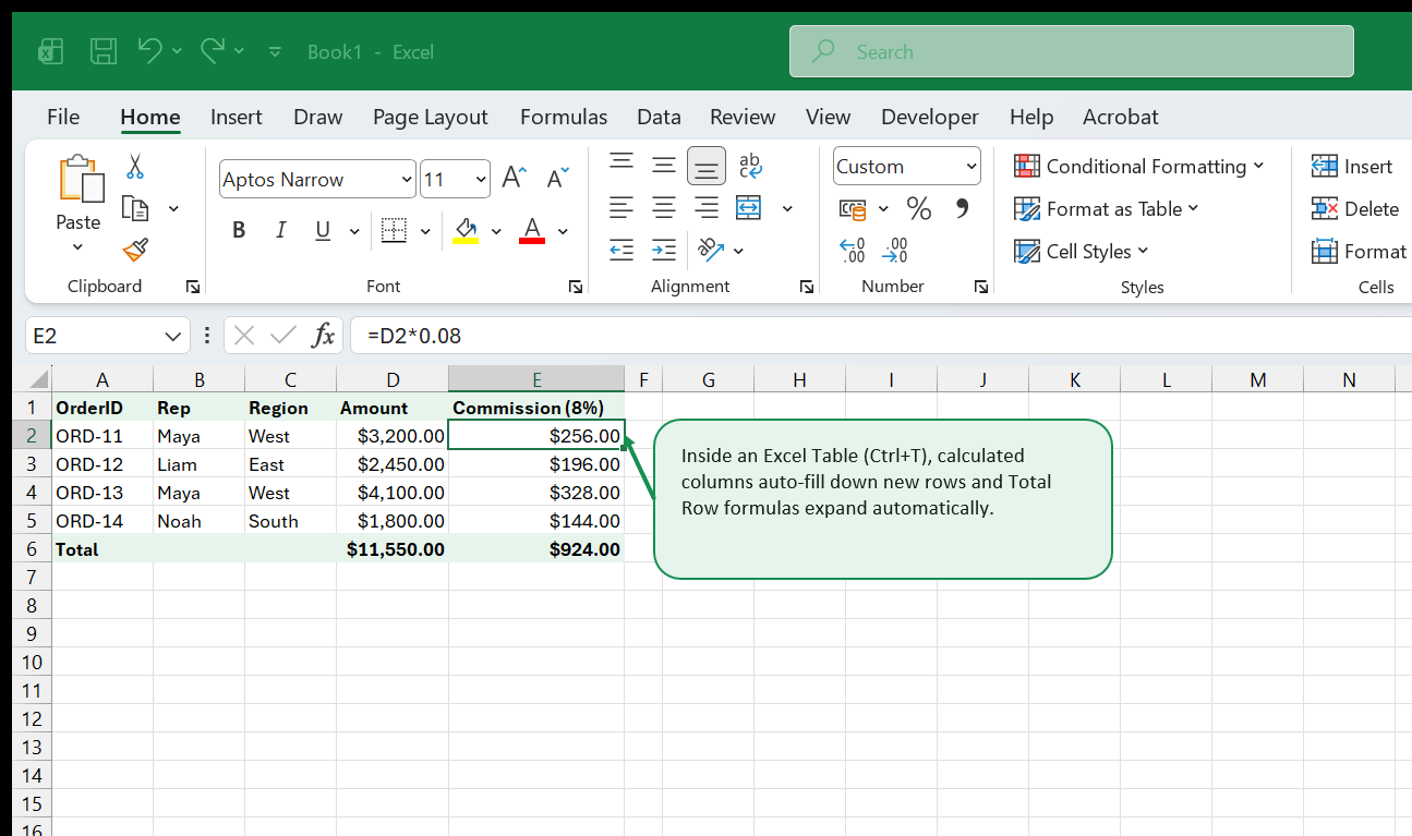
Five Everyday Superpowers Inside Ctrl + T
- Auto-Expanding Calculated Columns: Type a commission formula once in row 2 (
=D2*0.08or structured=[@Amount]*0.08) and press Enter — Excel copies it seamlessly down every row of the column without dragging the fill handle. - One-Click Total Row: Open Table Design → Total Row to toggle a clean bottom total bar with instant
Sum,Average,Count,Min, orMaxdropdowns per column. - Readable Table Names: Rename
Table1totblSalesunder Table Design → Table Name so downstream dashboards read=SUM(tblSales[Amount])instead of cryptic'Raw Sheet'!D2:D842. - Sticky Headers on Scroll: Scrolling down past row 40 automatically swaps
A, B, C, Dcolumn letters for your table’s real header names (OrderID,Rep,Region,Amount) without touching Freeze Panes. - Instant Slicers: Even without a PivotTable, Table Design → Insert Slicer lets teammates filter plain Excel Tables by clicking visual Region or Status cards!
2. Multi-Criteria Summaries with SUMIFS & COUNTIFS
Goal: Answer compound business questions (“Total Software sales in West”) in one readable formula without creating helper filter tabs.
Single-condition SUMIF handles "All West sales" easily, then falls short the instant a manager asks for "West AND Software". Moving straight to the plural functions — SUMIFS, COUNTIFS, and AVERAGEIFS — gives you unlimited paired conditions in one clean formula, even when you only have a single rule right now.

Watch the Argument Flip Between SUMIF and SUMIFS
Always put the sum range FIRST in SUMIFS (D2:D6), followed by alternating (criteria_range, criteria) pairs:
=SUMIFS(D2:D6, B2:B6, G2, C2:C6, G3)Pairing SUMIFS directly above COUNTIFS(B2:B6, G2, C2:C6, G3) puts both revenue ($7,700) and order volume (2 orders) on your summary block simultaneously so readers see average deal size (=G4/G5) instantly.
Using Comparison Operators & Wildcards Inside Criteria
Wrap greater-than/less-than operators in quotes concatenated with cell references: ">="&H1 sums only orders equal to or above threshold cell H1. Need partial text matches like "Pro*"? Combine wildcards (* for any characters, ? for single character) directly inside the quoted criterion.
3. Modern Lookups with XLOOKUP & Clean Error Fallbacks
Goal: Replace fragile VLOOKUP column counting with XLOOKUP, returning names, departments, and base pay safely with built-in "Not found" handling.
Countless beginner sheets break when someone inserts a new column inside a lookup table (VLOOKUP column index 3 suddenly reads column C instead of D, returning garbage quietly). Modern XLOOKUP selects the lookup column and return column independently, works right-to-left or left-to-right, and defaults safely to exact matching (0).
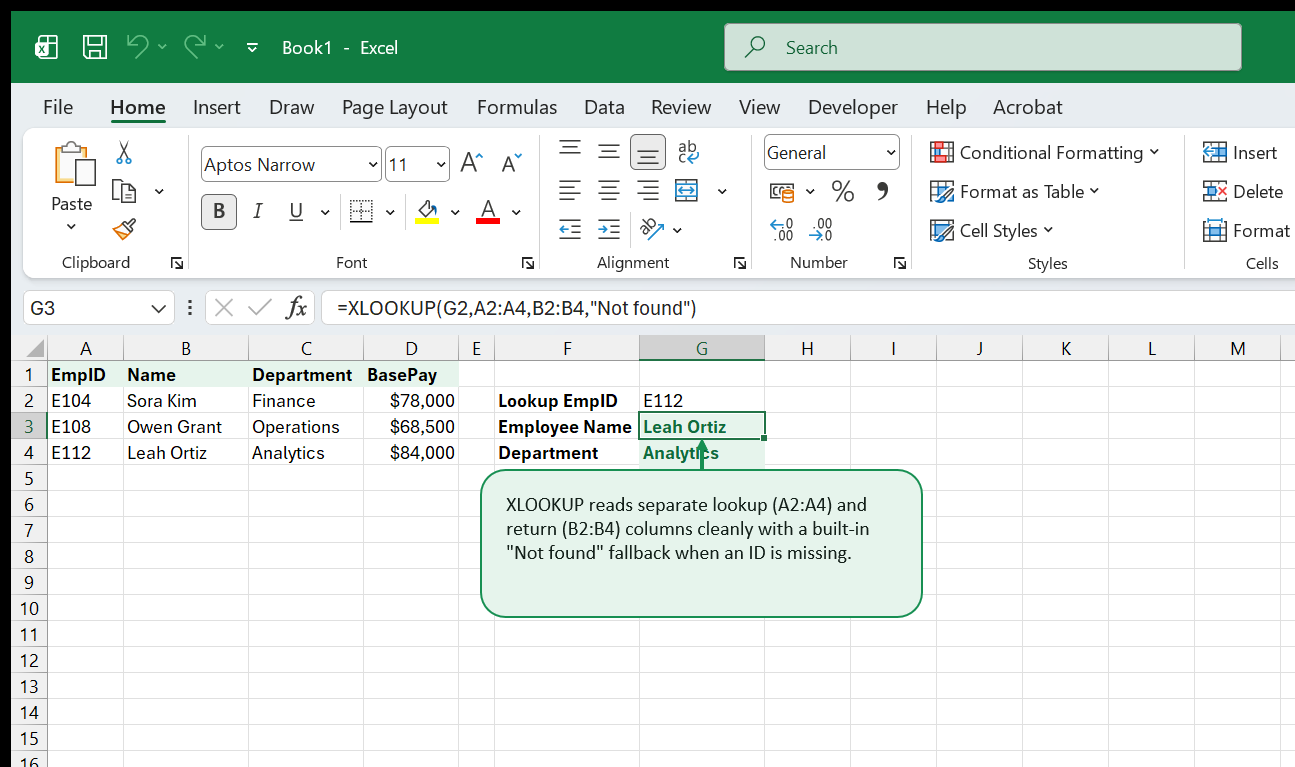
=XLOOKUP(G2, A2:A4, B2:B4, "Not found")Why Supplying Argument 4 (if_not_found) Is Mandatory Discipline
Leaving argument 4 blank surfaces harsh #N/A errors whenever a user enters a new employee ID that hasn’t reached HR payroll yet. Writing "Not found" (for text fields) or 0 (for additive currency totals) makes reports look intentional and keeps downstream =SUM(G5:G10) ranges calculating without #N/A cascades. Still supporting an older Excel 2016 teammate? Read INDEX & MATCH Deep Dive or the XLOOKUP Function Reference.
4. Bulletproof Task Trackers with Data Validation Dropdowns
Goal: Eliminate spelling drift ("Done " vs "done" vs "Completed") using controlled dropdown lists and helpful hover prompts.
A task dashboard counting "Done" with COUNTIF(D2:D50, "Done") misses "done " (trailing space), "Finished", and "Complete" silently. Data Validation enforces clean inputs right at entry time so formulas stay accurate forever.
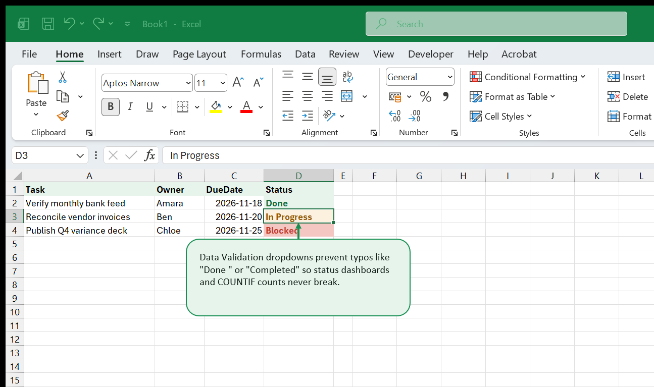
Setting Up Input Prompts & Error Alerts
Select D2:D25, open Data → Data Validation:
- Under Settings, choose Allow: List and supply clean items (
Not Started, In Progress, Blocked, Done) — or better yet, point to a maintenance range on aListstab (=$J$2:$J$5) so adding"In Review"updates every dropdown automatically. - Switch to Input Message: enter Title
"Choose Status"and message"Pick a standardized status so COUNTIF rollups stay exact."Now every teammate sees crisp guidance on click! - Set Error Alert → Style: Stop so invalid free-typing is cleanly blocked.
5. Clean Department Variance Tables & Executive Charts
Goal: Combine compact Budget vs. Actual variance tables with clean clustered column visuals that pass the five-second clarity test.
Long spreadsheets fatigue busy readers. Summarizing forty transaction tabs into one concise 4-column summary block paired beside a balanced chart communicates department health immediately.

Formatting Variance So Overspend Pops Immediately
Notice column D (=B2-C2): Budget minus Actual yields positive numbers when under budget and negative numbers (-$3,200) when Operations overspends. Apply accounting parentheses format ($#,##0;($#,##0);"-") alongside a simple Conditional Formatting highlight rule (Less Than 0 → Light Red Fill) so overspends jump off the page without squinting! See Conditional Formatting Mastery for complete formatting rules.
6. Readable Long Ledgers with Multi-Axis Freeze Panes
Goal: Lock header rows AND key ID/Date columns simultaneously using Freeze Panes at cell B2 (or C2) plus clean grid design.
Nothing ruins reviewing a 15-column vendor ledger faster than scrolling sideways to column M and forgetting which date or account row 84 belongs to. Most users click Freeze Top Row, forgetting that View → Freeze Panes → Freeze Panes freezes both rows above AND columns to the left of your active cursor cell!

Quick Cheat Sheet: Exact Cell to Click Before Freeze Panes
| Layout Goal | Click Cell | Rows Frozen | Columns Frozen |
|---|---|---|---|
| Keep header row only | A2 |
Row 1 | None |
Keep header + column A (Date) |
B2 |
Row 1 | Column A |
| Keep 2 title rows + columns A–B | C3 |
Rows 1–2 | Columns A–B |
7. Cleaning Sloppy Teammate Text with TRIM, PROPER & TEXTSPLIT
Goal: Repair ragged pasted customer names, mixed casing, and leading spaces in seconds instead of retyping rows manually.
External exports love sneaking trailing spaces ("Maya "), double internal spaces ("Maya Patel"), and all-caps names ("LIAM CHEN") into spreadsheets — breaking XLOOKUP and SUMIFS cleanly every time. Keep a fast 3-function repair toolkit ready:
=TRIM(PROPER(A2))PROPERcapitalizes first letters cleanly across names.TRIMstrips every leading, trailing, and duplicate middle space.CLEANdeletes invisible line-break control characters copied out of web forms. Need an instant fix outside Excel? Run lists through our CSV Cleaner Tool.
8. Date Math Without Calendar Guessing (EOMONTH, EDATE, NETWORKDAYS)
Goal: Compute invoice due dates, subscription renewals, and business SLA days accurately without counting weekends or 30/31-day months by hand.
Never type +30 or +365 for monthly contracts — leap years and 31-day months silently drift invoices off billing cycles. Excel’s calendar functions respect exact calendar lengths cleanly:
- Same day
Nmonths ahead:=EDATE(StartDate, 3)adds 3 calendar months cleanly (Jan 31→Apr 30). - Exact month-end billing cutoff:
=EOMONTH(InvoiceDate, 0)snaps to the last day of the current month;=EOMONTH(InvoiceDate, 1)jumps to the end of next month. - Business days excluding weekends (and optional holidays):
=NETWORKDAYS(StartDate, EndDate, HolidaysRange). Deepen your calendar fluency in Date & Time Functions Guide.
9. Multi-Condition Branching with IFS & Readability with LET
Goal: Untangle hard-to-read five-level nested IF(IF(IF(...))) formulas into clean vertical branches and reusable variable names.
Classic nested IF statements turn into parenthesis soup fast. Modern Excel’s IFS tests conditions strictly left-to-right without nesting parentheses, closing cleanly with a TRUE catch-all default at the end:
=IFS(D2="Done","Complete", C2<TODAY(),"Overdue", C2<=TODAY()+3,"Due Soon", TRUE,"On Track")Whenever a calculation repeats an expensive lookup twice, LET calculates it once inside a readable variable name — cutting sheet math in half and making formulas self-documenting!
10. Custom Number Formatting Tricks That Preserve Real Math
Goal: Display "30 days", +$1,450, (2.4%), or $14.2K visually while leaving cells 100% numeric for formulas and charts.
Typing "14 days" directly into a cell turns that cell into plain text — breaking SUM, AVERAGE, and charts instantly. Always enter bare numbers (14) and open Format Cells (Ctrl + 1) → Custom:
| Custom Format Code | Raw Cell Value | Displayed Value | Safe for SUM? |
|---|---|---|---|
0" days" |
14 |
14 days |
Yes |
+$#,##0;($#,##0);"–" |
-320 |
($320) |
Yes |
"$"#,##0,"K" |
14200 |
$14K |
Yes |
yyyy-mm-dd |
2026-11-14 |
2026-11-14 |
Yes |
11. Page Setup, Print Titles & Clean PDF Handoffs
Goal: Prevent embarrassing 1-column orphan page spills before exporting a spreadsheet to PDF or printing for a team meeting.
Nothing undermines hard spreadsheet analysis faster than sending a PDF whose rightmost column spills onto Page 2 with zero row headers. Spend thirty seconds under Page Layout before every share:
- Orientation & Scaling: Choose Landscape for wide tables and set Width: 1 page / Height: Automatic under Scale to Fit so columns never split horizontally across pages!
- Repeat Header Row on Every Printed Page: Open Page Layout → Print Titles → Rows to repeat at top and select
$1:$1. Now Pages 2, 3, and 4 all carry crisp table headers automatically. - Preview Cleanly: Switch to View → Page Break Preview (blue dashed lines) and drag breaks cleanly between sections rather than mid-table.
12. Workbook Safety & Your Next Excel Milestones
Goal: Protect formula ranges from accidental deletion while keeping user input cells unlocked, and chart your path forward across ExcelBack.
Before handing a tracker to teammates, unlock only the cells people should type into (Format Cells → Protection → uncheck Locked on input/dropdown ranges, shaded soft cream/blue as visual cues), then turn on Review → Protect Sheet. Collaborators pick dropdowns and update numbers effortlessly while every SUMIFS and XLOOKUP stays untouchable!
Continue Building Your Skills on ExcelBack
- Automate recurring CSV cleanup: Power Query Quick Start & Power Query & M Transformations (Volume 2) eliminate repetitive weekly formatting.
- Analyze thousands of rows dynamically: Pivot Tables from Zero & Pivot Tables & Data Models (Volume 2).
- Practice interactive formulas & workbooks: Download ready-to-use files on ExcelBack Templates, Datasets, and test formulas step by step in Formula Explainer.
13. Visual Highlighting Without Manual Painting (Quick Rules)
Goal: Flag overdue invoices, top 10% sales reps, and duplicate order IDs dynamically using Conditional Formatting inside your Excel Tables.
Manual Fill Color (yellow or light red) lies the instant numbers update next Monday. Replace static bucket painting with three foundational Home -> Conditional Formatting patterns inside everyday workbooks:
- Duplicate Value Check: Select Order ID column -> Highlight Cells Rules -> Duplicate Values… to expose accidental double-billing entries the moment you paste them.
- Threshold Alerts: Highlight
Days_Overdue > 0with light red fill, dark red text so past-due receivables stand out without squinting through rows. - In-Cell Data Bars: Select numeric revenue or progress % columns -> Data Bars -> Solid Fill so reviewers compare magnitudes visually without needing a separate bar chart!
Remember rule hygiene: press Conditional Formatting -> Manage Rules -> This Worksheet monthly to clear split fragmented ranges ($D$2:$D$14, $D$16:$D$40) created by sloppy copy-pasting.
14. Text Splitting & Cleanup Power Trio (TRIM, TEXTBEFORE, TEXTSPLIT)
Goal: Split "Maya Chen — Finance (Austin)" or messy CSV strings dynamically into separate clean columns without destructive Text-to-Columns re-runs.
Traditional Data -> Text to Columns snaps once and leaves stale text behind tomorrow when new rows arrive. Modern dynamic text formulas clean AND split live:
| Task | Clean Excel Formula | Example Result ("Maya Chen — Finance") |
|---|---|---|
| Remove stray extra spaces | =TRIM(A2) |
"Maya Chen — Finance" |
| Standardize Title Case | =PROPER(TRIM(A2)) |
"Maya Chen — Finance" |
| Grab text before delimiter | =TEXTBEFORE(A2, " — ") |
"Maya Chen" |
| Grab department after delimiter | =TEXTAFTER(A2, " — ") |
"Finance" |
| Split full CSV string across columns | =TEXTSPLIT(A2, ",") |
Spills horizontally cleanly |
If your office runs older Excel 2019 without TEXTBEFORE, combine LEFT(A2, FIND(" — ", A2) - 1) cleanly—or better, let Flash Fill (Ctrl + E) learn structural splits from two typed examples cleanly for one-off cleanup jobs!
15. Essential Date Arithmetic Without Weekend Mistakes
Goal: Calculate exact contract expiration dates (EDATE, EOMONTH) and true business days (NETWORKDAYS, WORKDAY) for billing and HR trackers.
Typed dates fail beginners most often during month-end rollovers (Jan 31 + 30 days = Mar 2 instead of Feb 28!). Use Excel’s calendar-aware date functions every time:
=EOMONTH(B2, 2)EOMONTH(start_date, months): Jumps straight to the exact final calendar dayNmonths forward (handling leap years and28/30/31-day months flawlessly!).EDATE(start_date, months): Adds exact anniversary months cleanly without drifting from the 15th onto the 14th or 16th.NETWORKDAYS(start, end, [holidays]): Counts business days excluding Saturdays, Sundays, and company holiday lists—essential for shipping SLAs and leave balances.
16. Keyboard Navigation Speedups That Double Daily Throughput
Goal: Replace slow mouse scrolling across multi-thousand-row workbooks with seven muscle-memory keystrokes.
Moving cleanly inside spreadsheets takes half the time when your right hand stays off the mouse scroll wheel:
Ctrl + Arrow Key: Jumps straight to the very top, bottom, left, or right edge of your contiguous data table (Ctrl + Downfinds row8,450in0.1seconds!).Ctrl + Shift + Arrow Key: Highlights all the way down/across cleanly for instant Totals, Charts, or Format Painting (Ctrl + Shift + Down).Ctrl + Space/Shift + Space: Selects an entire column (Ctrl + Space) or row (Shift + Space) cleanly, ready forCtrl + +to insert orCtrl + -to delete.Alt + =(AutoSum): Inserts=SUM(...)below or beside any numeric block instantaneously without typing a letter.Ctrl + 1: Opens Format Cells cleanly for custom accounting formats, alignments, and border edits.Ctrl + Shift + L: Toggles Filter dropdown arrows on/off across active header rows immediately.F4Repeat Action / Lock$: Repeats your previous formatting action outside the formula bar—and toggles$A$1absolute anchors inside the formula bar!
17. Multi-Sheet Summaries & Safe 3D Consolidation Habits
Goal: Combine January, February, and March tabs cleanly into a YTD Summary without fragile broken cross-sheet links.
When a workbook starts with separate monthly sheets (Jan, Feb, Mar) using identical row and column layouts, Excel supports fast 3D SUM references:
=SUM(Jan:Mar!D5)Even safer for growing organizations: avoid scattering identical transactions across twelve separate tabs altogether whenever possible! Keeping all twelve months inside one clean Master Ledger Table with an explicit Month column (2026-01, 2026-02, 2026-03) lets SUMIFS and PivotTables slice every month simultaneously with zero formula rewrites when April arrives.
18. Practice Project: Building the Complete Weekly Tracker From Zero
Goal: Combine Tables, XLOOKUP, SUMIFS, Data Validation, Freeze Panes, and a clean executive summary chart inside one unified 15-minute build.
Follow this end-to-end build sequence on any clean sales or expense export:
- Format Raw Sheet (
Ledger): Clean any stray summary rows, ensure ISO dates and real right-aligned currency decimals, then pressCtrl + T-> name TabletblLedger. - Guard Inputs: Apply Data Validation dropdowns (
Direct,Partner,Online) onChanneland positive decimal validation onAmount. - Add Dynamic Lookup: Create a small
Ownerslookup sheet mapping eachRegion->AccountLead, and bringAccountLeadintotblLedgerdynamically using@RegioninsideXLOOKUPwith"Unassigned"fallback. - Build
SummaryTab: Summarize totals perRegionandChannelcleanly viaSUMIFSreferencing structured columns (tblLedger[Amount]), add a crisp Clustered Column chart with takeaway title ("Online Leads Q2 Growth"), and verifySummary Total = SUM(tblLedger[Amount])equals$0.00variance! - Lock Print View: Freeze header row (
Alt + W + F + R), set Landscape Fit All Columns on One Page, and previewCtrl + P.
19. Everyday Skills Pre-Send Audit Checklist
Goal: Complete a 60-second quality sweep before emailing any Excel deliverable to managers, finance controllers, or clients.
| Audit Item | Quick Check Method | Pass Standard |
|---|---|---|
Zero # Error Codes |
F5 -> Special -> Formulas -> Errors |
Selection returns “No cells were found” |
| Zero Accidental Hardcodes | Toggle Ctrl + ~ (Show Formulas) |
Total rows show green formulas cleanly, not typed integers |
| Control Totals Tie | Subtract Summary Grand Total - Raw Total |
Variance cell displays $0.00 (Check = OK) |
| Clean Print Layout | Press Ctrl + P preview across all tabs |
No cut-off columns, no ### overflow hashes, crisp headers |
| Cursor Parked Cleanly | Select cell A1 on Summary tab before Save |
File opens cleanly at top-left summary view for recipients |
Building these everyday table, lookup, summary, and verification habits transforms Excel from an error-prone scratchpad into a calm, dependable system you trust completely under deadline pressure.
20. Hands-On Practice Lab: End-to-End Department Expense Tracker
Goal: Apply Excel Tables, XLOOKUP category mapping, multi-condition SUMIFS, Data Validation menus, and Conditional Formatting together inside a real department budget review sheet.
Recreate this complete 4-tab mini-workbook cleanly from scratch to lock in Volume 2 habits:
Catalog_ListsTab: Enter five clean spending categories (Software,Hardware,Travel,Training,Supplies) and quarterly budget caps beside each ($18,000,$12,000,$9,500,$6,000,$4,000), then pressCtrl + Tto name the TabletblBudgets.ExpensesLedger Tab: Create headersDate | Vendor | Category | Description | Amount | ApprovalCode-> convert totblExpenses(Ctrl + T). Apply Data Validation (List) onCategoryreading=tblBudgets[Category]so zero invalid category names ever slip into rows!SummaryTab: List each Category cleanly inA5:A9. Compute Actual Spend inB5using=SUMIFS(tblExpenses[Amount], tblExpenses[Category], A5), pull Quarterly Budget inC5via=XLOOKUP(A5, tblBudgets[Category], tblBudgets[Cap], 0), and compute Remaining Headroom (=C5-B5).- Alerts & Visual Polish: Highlight
Remaining Headroom < 0in soft red via Conditional Formatting, turn on Freeze Panes on Row5ofSummary, and verifySUM(B5:B9) - SUM(tblExpenses[Amount]) = $0.00reconciliation tie-out cleanly!
21. Everyday Office Formula & Keyboard Reference Card
Goal: Bookmark Volume 2’s essential multi-criteria formulas and everyday speed keys cleanly for fast desktop recall.
| Everyday Requirement | Production Formula Pattern | Key Advantage Over Basics |
|---|---|---|
| Sum with 2+ filters | =SUMIFS(Amount, Region, "West", Year, 2026) |
Handles up to 127 criteria cleanly with dynamic ranges |
| Count matching multiple tags | =COUNTIFS(Status, "Active", Owner, A2) |
Never breaks when inserting columns |
| Clean missing lookup safely | =XLOOKUP(A2, SKUList, PriceList, "Missing") |
Replaces fragile VLOOKUP index counts & #N/A errors |
| Safe multi-tier categorization | =IFS(Rev>=10000,"Tier 1", Rev>=5000,"Tier 2", TRUE,"Core") |
Eliminates unreadable nested IF(IF(IF(...))) chains |
| Month-end target billing date | =EOMONTH(StartDate, 2) |
Automatically handles 28/29/30/31-day month lengths |
Keep Ctrl + T (Tables), Ctrl + Shift + L (Filter toggles), Ctrl + ~ (Show Formulas), and Alt + W + F + F (Freeze Panes) ready on every morning workbook—small mechanical habits compound into hours saved every single week.
That's the whole book. Keep the PDF for offline reading.
Downloading requires a free Google sign-in -- reading online never does.